ABAP (Advanced Business Application Programming)

ABAP (Advanced Business Application Programming) is the primary programming language supported on the SAP NetWeaver ABAP application server platform and applications that run on it, such as SAP ERP (formerly R/3), S/4HANA and CRM.
SAP uses ABAP to implement its own applications on the NetWeaver ABAP platform, and SAP customers use ABAP to modify the functionality of SAP applications or build their own on the NetWeaver ABAP platform. ABAP is the oldest and, likely, the most widely used of SAP's four major application platforms, which also includes SAP NetWeaver Java, SAP Hana and SAP Cloud Platform.
Evolution of ABAP
SAP ABAP began in the 1980s as a report-generation language in SAP products. It took on a central role in SAP R/3 as the enterprise resource planning (ERP) system's primary implementation and extension language. Over the years, it gained new features, most notably the introduction of object-oriented constructs, referred to as ABAP Objects, in 1999 and the introduction of new database access methods and a large amount of new syntax starting around 2010.
ABAP features are tightly coupled with the SAP R/3 or NetWeaver release that is being used. The only way to access new features of the language is to upgrade to a newer release of the ABAP application server. In many cases, programs written using features of a newer application server version will not run on older SAP systems.
ABAP development tools
By far the largest developer of ABAP code is SAP itself. However, many thousands of ABAP developers work with SAP customers and consulting companies to maintain and modify SAP systems. ABAP is regularly in the top 30 of the Tiobe Index, which roughly tracks the popularity of programming languages.
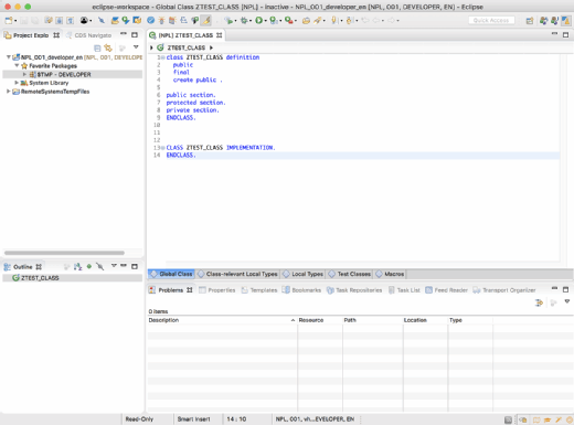
Developers who work in ABAP usually do so either in the ABAP Development Tools (a set of plug-ins for the Eclipse open source Java development platform) or in the ABAP Workbench transaction in the SAP graphical user interface (GUI). Both environments offer a set of tools to assist development, from code completion to automated testing tools.
SAP Solution Manager also offers tools for managing the development lifecycle of ABAP code. There is little support for development tooling beyond what SAP provides, though some customers have built their own integrations with third-party continuous integration, version control and bug tracking tools.
Special features and the larger ABAP infrastructure
ABAP doesn't stand alone, and it is highly integrated with other features of the SAP NetWeaver ABAP application server. Among these are the following:
- Logical database connections, which allow code to be abstracted from a specific database. The actual database connections are configured outside of ABAP code, allowing the same code to be used in different database environments.
- Open SQL, an abstraction of SQL syntax that is part of the ABAP language and which the ABAP runtime environment converts to native SQL that is appropriate for the database being used. Open SQL has many similarities to Microsoft .NET's Language Integrated Query (LINQ) concept.
- Internal Tables, which hold collections of objects that are accessed using special language keywords or Open SQL. This ABAP concept contrasts with the concept of typed arrays like in Java or C++.
- Security, in which ABAP is integrated with SAP NetWeaver's security infrastructure.
- Data Dictionary, a universal dictionary of data structure definitions, often including business logic, which is available to all ABAP programs in a system.
- Change and Transport System (CTS), which tracks changes to development objects and manages the promotion of development objects to quality assurance and production environments.
- Shared development system, which is an important aspect of ABAP. ABAP differs from most newer languages in that development usually takes place on a shared system, with all developers working on the same set of development objects at the same time.
ABAP and HANA
ABAP continues to be an important part of SAP's technology stack.
Though it has played a reduced role in many products with the advent of the HANA platform, it is still central to SAP's most widely deployed products, plays an important role in SAP's next-generation S/4HANA ERP platform and has been announced as a runtime for the SAP Cloud Platform.