Discover 2 unsupervised techniques that help categorize data

Category discovery: Overview

• Requirement. How can data be categorized into meaningful groups when the groups are not known in advance?
• Problem. Knowing plausible categories to which data might belong is not always possible, which makes it impossible to use classification algorithms to categorize data into relevant categories.
• Solution A clustering model is built that automatically groups similar data points into the same categories based on the intrinsic similarities between data attributes.
• Application. Clustering algorithms -- like K-means, K-medians and hierarchical clustering -- build the clustering model that organizes the data points into homogenous categories.

Category discovery: Explained

Problem

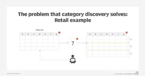
With data mining and exploratory data analysis, there is little information available about the makeup of data at hand. One example is a data set that contains data describing the shopping habits of online customers of an e-commerce retailer. The lack of knowledge about the groups to which different instances may belong and the lack of grouping examples renders the use of supervised machine learning techniques impossible. The objective, therefore, may be to find out if any natural customer groups exist, with the end goal of finding the characteristics of each group (Figure 1).

Solution

The data set is exposed to clustering, an unsupervised machine learning technique. This involves dividing data into different groups so the data in each group has similar properties. There is no prior learning of categories required. Instead, categories are implicitly generated and subsequently named and interpreted, based on the data groupings. How the data is grouped depends on the type of algorithm used.

Each algorithm uses a different technique to identify clusters. Once the groups are found, instances belonging to the same group are considered to be similar to each other. These groups can be further analyzed to gain a better understanding of their makeup and to determine why instances were allocated to different groups.

Clustering results can be used to preprocess data for semi-supervised learning, where class labels are first created based on the resulting groups, and the instances belonging to each group are then assigned the corresponding class labels. The labeled data can then be used for classification.

While clustering automatically creates homogeneous groups, the machine-generated labels often carry no real meaning. Humans must analyze the properties of each group and create meaningful labels as per the nature of the data analysis task, the business domain or the individuals to which the data mining results must be communicated.

Application

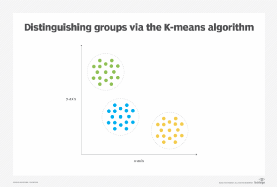
K-means is a common clustering algorithm that uses distance as a measure for creating clusters of homogeneous items. K is a user-defined number that denotes the number of clusters needed to be created and means refers to the center point of the cluster, or centroid. The centroid forms the basis for cluster creation around which other similar items that make up a cluster are located; it is determined from the mean of all point locations that represent the cluster items in a multidimensional space whose number of dimensions depends on the number of features of items to cluster. The value of K must be set within 1 ≤ K ≤ n, where n is the total number of items in the data set.

K-means is similar to K-nearest neighbors, in that it generally uses the same Euclidian distance calculation for determining closeness between the centroid and the items (represented as points) that requires the user to specify the K value (Figure 2). Operating in an iterative fashion, K-means begins with less homogeneous groups of instances and modifies each group during each iteration to attain increased homogeneity within the group. The process continues until maximum homogeneity within the groups and maximum heterogeneity between the groups is achieved.

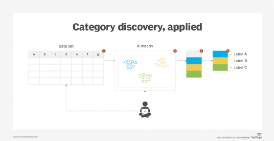
The category discovery pattern requires the application of the feature encoding pattern, as the category discovery pattern involves distance measurement, which requires all features to be numerical in nature. The application of the feature standardization pattern also ensures none of the large magnitude features overshadow smaller magnitude features in the context of distance measurement. In addition, the application of the feature discretization pattern helps reduce the feature dimensionality, which contributes to faster execution and increased generalizability of the model (Figure 3).

Pattern discovery: Overview

• Requirement. How can repeated sequences be found in large data sets made up of a number of features without any previous examples of such sequences?
• Problem. The discovery of naturally occurring groups within data is helpful with understanding the structure of the data. However, this does not help find meaningful repeating patterns within the data that can represent business opportunities or threats.
• Solution. An associative model is developed that identifies patterns within the data in the form of rules; these rules signify the relationship between data items.
• Application. Associative rule learning algorithms, such as Apriori and Eclat, are employed to build an associative model that extracts rules (patterns) based on how frequently certain data items appear together.

Pattern discovery: Explained

Problem

A data set can contain sequences of data that repeat themselves. These sequences are different from groups. In groups, one data item can only appear in one group, and there is no concept of ordering between the data items. In contrast, sequences represent data items that appear over and over again with some implicit ordering between all or a few elements of the sequence.

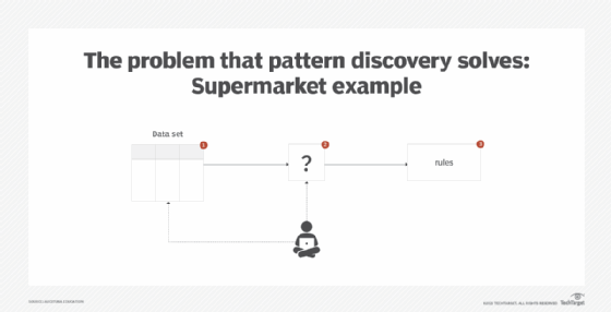
The identification of such repeating sequences can be of value to a business, such as finding co-occurring symptoms that lead to a fault. However, in such a scenario, regression, classification or clustering techniques are not applicable (Figure 4).

Solution

Association rules are extracted from the data set by first finding the repeating groups that are above a certain threshold value. Then, patterns in the form of association rules -- "if, then" relationships, in other words -- are extracted from the filtered repeating groups.

An association rule describes the relationship among items in a set. For example, milk, eggs and bread appearing in a single customer transaction at a grocery store are an item set, which is represented as {milk,eggs,bread}. A rule is generated from a subset of an item set and is generally written as X → Y, where X is the antecedent and Y is the consequent. A concrete example of an association rule is {milk,eggs} → {bread}, where the rule is read as milk and eggs infer bread. Or, in other words, a customer is likely to buy bread if milk and eggs are being purchased.

The significance of an association rule can be determined via the support, confidence and lift measures. Support measures the percentage of times a rule (both its antecedent and consequent) or an item set is matched within all transactions or rows of a data set.

Confidence measures the accuracy of the rule by dividing the support for the rule by the support of its antecedent (items only in the antecedent part of the rule). It should be noted that confidence (X → Y) is not same as its converse confidence (Y → X), as summarized with the following statement: confidence (X → Y) ≠ confidence (Y → X).

Lift measures the strength of the rule or the increase in value. It is measured by dividing the confidence for the rule by the support of its consequent. It compares Y occurring on its own against Y occurring as a result of X.

To determine whether a rule is meaningful or not, minimum threshold values are set for support and confidence. Rules that have support and confidence values above the minimum threshold values are considered meaningful and are called strong rules.

Application

A common algorithm for finding association rules among large data sets is the Apriori algorithm. The Apriori algorithm works on the heuristic known as the Apriori property, which states that all nonempty subsets of a frequent item set must also be frequent. For example, for {coffee,tea} to be frequent, both {coffee} and {tea} must also be frequent. Otherwise, this item set is excluded from rule generation (Figure 5).

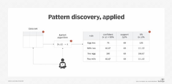
The Apriori algorithm uses support and confidence thresholds to decide which frequent item sets to search for in order to generate strong rules comprising the following two stages:

Stage 1: All frequent item sets whose support value is greater than or equal to the preset minimum threshold support value are found. It is based on iterative search, called level-wise search, where the algorithm starts by searching 1-member to n-member frequent item sets that are equal to or greater than the threshold support value.

Stage 2: Rules are created from the frequent item sets whose confidence value is equal to or greater than the preset minimum threshold confidence value.

This pattern requires the application of the feature discretization pattern, as the Apriori algorithm only works with nominal features.

What's next

The next article covers model evaluation techniques, including the training performance evaluation, prediction performance evaluation and baseline modeling patterns.