
Getty Images
ML model optimization with ensemble learning, retraining
Making ML models better post-deployment can be accomplished. Learn the ins and outs of two key techniques: ensemble learning and frequent model retraining.
This article is excerpted from the course "Fundamental Machine Learning," part of the Machine Learning Specialist certification program from Arcitura Education. It is the eleventh part of the 13-part series, "Using machine learning algorithms, practices and patterns."
Model optimization techniques are used to improve the performance of machine learning models. This and the next, final article in this series cover a set of optimization techniques that are normally applied toward the end of a machine learning problem-solving task, after a given model has been trained but when there exist opportunities to make it more effective.
This article describes the first two of four optimization practices: the ensemble learning and the frequent model retraining techniques. As explained in Part 4, these techniques are documented in a standard pattern profile format.
Ensemble learning: Overview
- How can the accuracy of a prediction task be increased when different prediction models provide varying levels of accuracy?
- Developing different models either using the same algorithm with varied training data or using different algorithms with the same training data often results in varied level of model accuracy, which makes using a particular model less than optimal for solving a machine learning task.
- Multiple models are built and used by intelligently combining the results of the models in such a way that the resulting accuracy is higher than any individual model alone.
- Either homogeneous or heterogeneous models (for classification or regression) are developed. Techniques such as bagging, boosting or random forests are then employed to create a meta-model.
Ensemble learning: Explained
Problem
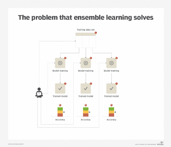
In the context of a classification or regression task, different models carry different strengths depending on whether they are trained using the same or different algorithms, and capture different aspects and relationships hidden in a data set. Even if the model with the highest accuracy is chosen, there is no guarantee that it will generalize well when exposed to unseen data in the production environment. Consequently, relying on a single model generally results in fluctuating accuracy based on whether the model sees the same type of unseen data that it is good at predicting. (See Figure 1.)
Solution
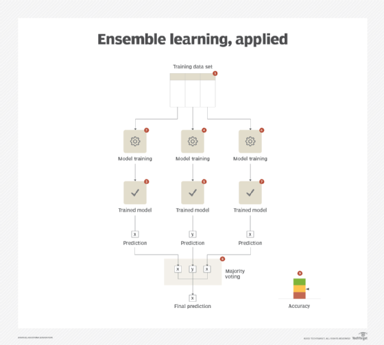
A single meta-model is generated that builds upon the strengths of each of its constituent models. The constituent models can be generated either by using the same type of algorithm for all models (each model differs in terms of its parameters) or different algorithms (applicable to the same type of machine learning problem, such as regression or classification) for each model. The results of all the constituent models are combined together using strategies such as voting or averaging. The meta-model works best when the constituent models carry a high accuracy but disagree among themselves as voting or averaging the same set of results does not bring any added value when compared with the results obtained from a single model.
Application
This pattern can be applied via one of the following strategies for creating a meta-model:
- Bagging. Bagging is short for bootstrap aggregating. The same algorithm is used to train multiple models in parallel such that each is trained on a subset of the training data constructed by bootstrap sampling. Bootstrap sampling is a sampling method where a sample is generated by randomly selecting, with replacement items, from a data set. That is, each time an item is selected, it is returned to the data set. Therefore, it is possible that the same item can be selected more than once for the same sample. The meta-model is generated by aggregating the results of different models either via voting (classification task) or averaging (regression task). A specialized form of bagging is random forests, whereby the underlying algorithm for constituent models is a decision tree. However, each tree is exposed to a different subset of features that results in randomized trees, which upon aggregation provides a better accuracy than each of the constituent trees.
- Boosting. Boosting is a sequential ensemble technique that transforms low-accuracy models (weak learners) into a strong ensemble model. A simple model with low accuracy is first trained, and the next version of the model then concentrates on those instances of the training data set that were incorrectly classified. Each successive version of the model is trained using the complete training data set. In the end, the predictions from each model are combined into a single final prediction via weighted majority voting (classification task) or weighted sum (regression task).
The ensemble learning pattern can further benefit from the application of the baseline modeling pattern. With an established baseline, it is easier to select the right combination of constituent models. (See Figure 2.)
Frequent model retraining: Overview
- How can the efficacy of a model be guaranteed after its initial deployment?
- After a model is deployed to the production environment, there is a strong possibility that the accuracy of the model may decrease over time, resulting in degraded system performance.
- The machine learning model is kept in sync with the changing data by keeping the model up to date.
- The model is retrained at regular intervals by preparing a training data set that includes both historic data as well as the current data.
Frequent model retraining: Explained
Problem
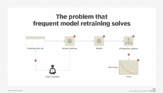
Once a model has been developed and tested to provide valuable insights, it is deployed in the production environment. However, over time, the model does not remain as accurate as it was when it was first deployed and provides less accurate results. With a classification model, the false positive or false negative rate may increase. With a regression model, the mean squared error (MSE) may increase. [Editor's note: MSE is a measure that determines how close the line of best fit is to the actual values of the response variable. See Part 9 of this series for a further explanation.] The increase of MSE suggests the model is losing its efficacy, which can result in lost business opportunities or the inability to address a threat in a timely manner. (See Figure 3.)
Solution
The decrease in the efficacy of a model after its initial deployment can be attributed to the changing nature of the input data, which itself can be traced back to a change in the data-generating process. To keep up with these changes, the model is periodically refreshed. This involves preparing a training data set that is comprised of both the current and historical data, then retraining the model. Periodic retraining of the model ensures that the model keeps capturing the true concept the data encompasses and thus remains accurate.
Application
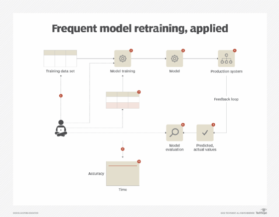
The application of this pattern is dependent upon the existence of a feedback loop that informs on the effectiveness of the model. This requires setting up a process that records the predicted and actual values, keeping in mind that the actual values will only be available after the fact. For model retraining, a representative data set needs to be gathered to include a blend of both newly observed data and historic data. Based on the nature of the business problem at hand, either the same algorithm can be reused for the next iteration or a different algorithm can be used. The latter generally happens if the current algorithm is unable to fully capture the underlying concept and the error rate keeps increasing when retrained with new data. If the same algorithm suffices, the entire model retraining process can be automated. However, in both the cases, it is vital that the performance of the model is tracked on a continuous basis.
As retraining a model from scratch can consume valuable time and effort, the frequent model retraining pattern can further benefit from the application of the incremental model learning pattern (covered in the next article), provided that fit-for-purpose algorithmic implementations are available for the task at hand (Figure 4).
What's next
The next article covers the second pair of model optimization techniques: the lightweight model implementation and the incremental model learning patterns.
View the full series
This lesson is one in a 13-part series on using machine learning algorithms, practices and patterns. Click the titles below to read the other available lessons.
Lesson 1: Introduction to using machine learning
Lesson 2: The "supervised" approach to machine learning
Lesson 3: Unsupervised machine learning: Dealing with unknown data
Lesson 4: Common ML patterns: Central tendency and variability
Lesson 5: Associativity, graphical summary computations aid ML insights
Lesson 6: How feature selection, extraction improve ML predictions
Lesson 7: 2 data-wrangling techniques for better machine learning
Lesson 8: Wrangling data with feature discretization, standardization
Lesson 9: 2 supervised learning techniques that aid value predictions
Lesson 10: Discover 2 unsupervised techniques that help categorize data
Lesson 11
Lesson 12: 3 ways to evaluate and improve machine learning models
Lesson 13: Model optimization methods to cut latency, adapt to new data