Wrangling data with feature discretization, standardization

Feature discretization: Overview

• How can continuous features be used for model development when the underlying machine learning algorithm only supports discrete/nominal features? Or: How can the range of values that a continuous feature can take on be reduced in order to lower model complexity?
• Some machine learning algorithms can only accept discrete or nominal features as input, which makes the inclusion of valuable continuous features impossible as an input for model development. Or: Using numerical features with a very wide range of continuous values makes the model complicated with further implications of overfitting and longer training and prediction times.
• A limited number of discrete sets of values are derived from continuous features by employing statistical or machine learning techniques.
• The continuous features are subjected to techniques such as binning and clustering that group continuous values into discrete bins, thereby discretizing continuous features into discrete ones.

Feature discretization: Explained

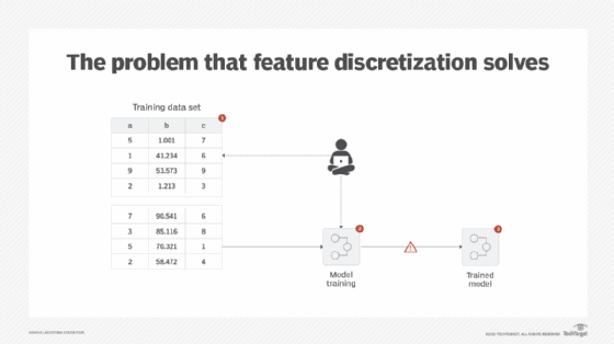
Some non-distance-based machine learning algorithms -- in other words, those that do not use distance measure for classification or clustering such as Naïve Bayes -- normally require input to comprise only categorical or discrete values. Even if an algorithm is able to work with continuous values, with the possibility of a very large number of feature values such as slight variations in decimal values of temperature readings with four decimal places, the dimension of the feature space becomes unwieldly. This makes the underlying mathematical operations too expensive. For example, with Naïve Bayes, the algorithm needs to calculate the probability of each unique value, which can be far too many in cases with large data sets with decimal values. This results in long training and prediction times (Figure 1).

Solution

The continuous values are reduced to a manageable set of discrete values, such as ordinal or categorical values. The reduction is either achieved by a simple binning strategy, such that values in a certain range get replaced by the label of the corresponding bin, or by a more complex operation involving the use of other features such that the values grouped closely in n-dimensions are allocated to a single ordinal value.

Application

A number of techniques can be applied to achieve discretization, including binning and clustering.

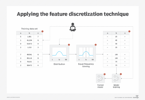
Binning is where ordered attribute values are grouped into intervals or bins, which can be created using either the equal-frequency or equal-width methods. The bin labels can be used in place of the original attribute values. This technique is affected by outliers and skewed data. In the equal-width method, the interval of values is the same, with each bin generally containing a different number of values. In the equal-frequency method, each bin contains the same number of values so the interval of values is generally not the same. To determine which type of binning to use, it is recommended to look at the shape of the distribution. With a Gaussian distribution, equal-frequency binning is normally used, whereas equal-width binning is normally used for a uniform distribution.

Clustering involves the use of a clustering algorithm to divide a continuous attribute into a set of groups, based on the closeness and distribution makeup of the attribute values. Using clustering, outliers can be detected to prevent adverse effects of outliers on data discretization (Figure 2).

Feature standardization: Overview

• How can it be ensured that features with wide-ranging values do not overshadow other features carrying a smaller range of values?
• Features whose values exist over a widescale carry the possibility of reducing the predictive potential of features whose values exist over a narrow scale, thereby resulting in the development of a less accurate model.
• All numerical features in a data set are brought within the same scale so that the magnitude of each feature carries the same predictive potential.
• Statistical techniques, such as min-max scaling, mean normalization and z-score standardization, are applied to convert the features' values in such a way that the values always exist within a known set of upper and lower bounds.

Feature standardization: Explained

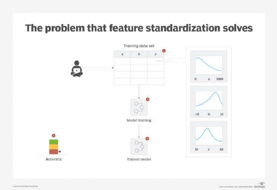
A data set may contain a mixture of numerical features where some features operate at a different scale, such as one feature with values between -100 to +100 and another feature with values between 32 and 212. There can also be a difference in the units used by different features, such as one feature using meters while another uses kilometers. These differences incorrectly give more importance to features with higher magnitudes than lower ones. As a result, algorithms using distance calculation, such as Euclidean distance, focus on features with higher magnitudes and ignore the contribution of smaller magnitude features. In addition, a unit change in a feature using smaller units, such as yards, is treated the same as the feature using bigger units, such as miles, which should not be the case (Figure 3).

Solution

All numerical feature values are transformed so that there is no difference in magnitude and they operate within the same scale. Two different techniques exist for standardization: scaling and normalization. Scaling modifies the range of the data and is used when the distribution is non-Gaussian or when there is uncertainty about the type of distribution. Normalization modifies the shape of the data (distribution) and transforms it into a normal distribution. It is used when the data is Gaussian in nature and the algorithm for model training requires input data to be in normal form.

Application

Both scaling and normalization are generally applied using data preprocessing functions available either within the model development software or as a separate library that can be imported.

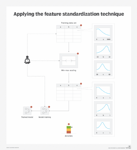
For scaling, a popular algorithm is min-max scaling, which brings the values within 0 and 1. However, based on requirements, another practice is to scale data between -1 and +1.

For normalization, either z-score standardization or mean normalization can be used. Z-score standardization transforms the values into a distribution with zero mean and unit standard deviation, while mean normalization transforms the values into a distribution with zero mean and a range from -1 to +1 (Figure 4).

What's next

The next article covers two supervised learning patterns: numerical prediction and category prediction.