2 supervised learning techniques that aid value predictions

Numerical prediction: Overview

• Requirement. How can the value of a numerical variable be predicted based on a set of known values of other variables?
• Problem. Certain machine learning problems require predicting a numerical value based on some known variables, making it impossible to apply machine learning techniques where the target can only be a categorical variable.
• Solution. The relationship between the known variables and the target variable is captured using a regression algorithm, which is then used to predict the unknown value of the target variable based on known values of the other variables.
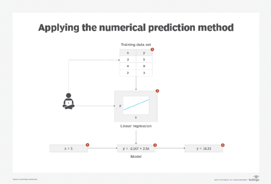
• Application. Regression algorithms, such as linear regression, are applied to the data set by first developing a model based on the known set of values of both the target and other variables, and then making predictions for the unknown value of the target variable based on a known set of values of other variables.

Numerical prediction: Explained

Problem

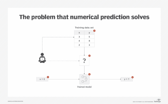
A data set may contain a number of historical observations (rows) amassed over a period of time where the target value is numerical in nature and is known for those observations. An example is the number of ice creams sold and the temperature readings, where the number of ice creams sold is the target variable. To obtain value from this data, a business use case might require a prediction of how much ice cream will be sold if the temperature reading is known in advance from the weather forecast. As the target is numerical in nature, supervised learning techniques that work with categorical targets cannot be applied (Figure 1).  

Solution

The historical data is capitalized upon by first finding independent variables that influence the target dependent variable and then quantifying this influence in a mathematical equation. Once the mathematical equation is complete, the value of the target variable is predicted by inputting the values of the independent values.  

Application

The data set is first scanned to find the best independent variables by applying the associativity computation pattern to find the relationship between the independent variables and the dependent variable. Only the independent variables that are highly correlated with the dependent variable are kept. Next, linear regression is applied.

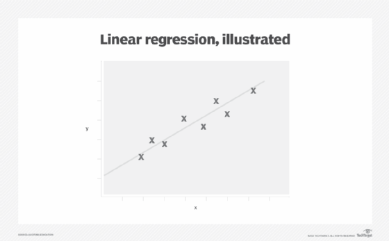
Linear regression, also known as least squares regression, is a statistical technique for predicting the values of a continuous dependent variable based on the values of an independent variable. The dependent and independent variables are also known as response and explanatory variables, respectively. As a mathematical relationship between the response variable and the explanatory variables, linear regression assumes that a linear correlation exists between the response and explanatory variables. A linear correlation between response and explanatory variables is represented through the line of best fit, also called a regression line. This is a straight line that passes as closely as possible through all points on the scatter plot (Figure 2).

Linear regression model development starts by expressing the linear relationship. Once the mathematical form has been established, the next step is to estimate the parameters of the model via model fitting. This determines the line of best fit achieved via least squares estimation that aims to reduce the sum of squared error (SSE). The last stage is to evaluate the model either using R squared or mean squared error (MSE).

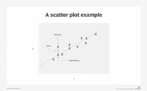
MSE is a measure that determines how close the line of best fit is to the actual values of the response variable. Being a straight line, the regression line cannot pass through each point; it is an approximation of the actual value of the response variable based on estimated values. The distance between the actual and the estimated value of response variable is the error of estimation. For the best possible estimate of the response variable, the errors between all points, as represented by the sum of squared error, must be minimized. The line of best fit is the line that results in the minimum possible sum of squares errors. In other words, MSE identifies the variation between the actual value and the estimated value of the response variable as provided by the regression line (Figure 3).

The coefficient of determination, called R squared, is the percentage of variation in the response variable that is predicted or explained by the explanatory variable, with values that vary between 0 and 1. A value equal to 0 means that the response variable cannot be predicted from the explanatory variable, while a value equal to 1 means the response variable can be predicted without any errors. A value between 0 and 1 provides the percentage of successful prediction.

In regression, more than two explanatory variables can be used simultaneously for predicting the response variable, in which case it is called multiple linear regression.

The numerical prediction pattern can benefit from the application of the graphical summaries computation pattern by drawing a scatter plot to graphically validate if a linear relationship exists between the response and explanatory variables (Figure 4).

Category prediction: Overview

• Requirement. How can the category that new data belongs to be predicted based on previous example data given so that the target categories are known in advance?
• Problem. In certain scenarios, the possible categories to which a data instance belongs to are known in advance along with examples of data instances belonging to these categories. However, what is not known is how to categorize new data instance into one of the known categories.
• Solution. A classification model is trained by using the example data in order to build an understanding of the characteristics of examples that belong to different categories. The model is then used to classify new instances into one of the known categories.
• Application. Classification algorithms such as KNN, naive Bayes, and decision trees are employed to build the classification model using existing example data and to predict the category of the new data instance.

Category prediction: Explained

Problem

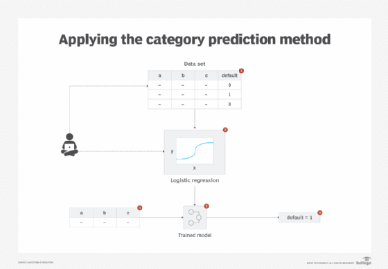
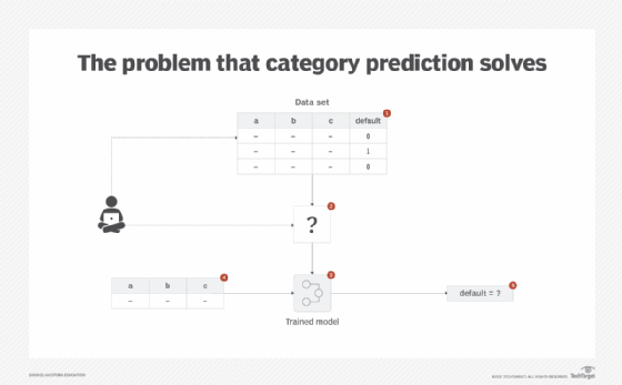
There are cases where a business problem involves predicting a category -- such as whether a customer will default on their loan or whether an image is a cat or a dog -- based on historical examples of defaulters and cats and dogs, respectively. In this case, the categories (default/not default and cat/dog) are known in advance. However, as the target class is categorical in nature, numerical predictive algorithms cannot be applied to train and predict a model for classification purposes (Figure 5).  

Solution

Supervised machine learning techniques are applied by selecting a problem-specific machine learning algorithm and developing a classification model. This involves first using the known example data to train a model. The model is then fed new unseen data to find out the most appropriate category to which the new data instance belongs.  

Application

Different machine learning algorithms exist for developing classification models. For example, naive Bayes is probabilistic while K-nearest neighbors (KNN), support vector machine (SVM), logistic regression and decision trees are deterministic in nature. Generally, in the case of a binary problem -- cat or dog -- logistic regression is applied. If the feature space is n-dimensional (a large number of features) with complex interactions between the features, KNN is applied. Naive Bayes is applied when there is not enough training data or fast predictions are required, while decision trees are a good choice when the model needs to be explainable.

Logistic regression is based on linear regression and is also considered a class probability estimation technique, since its objective is to estimate the probability of an instance belonging to a particular class.

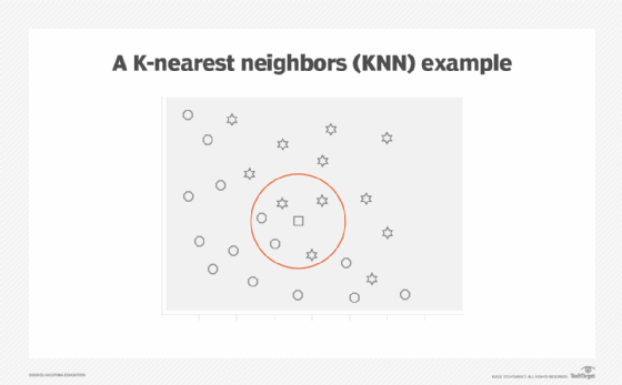
KNN, also known as lazy learning and instance-based learning, is a black-box classification technique where instances are classified based on their similarity, with a user-defined (K) number of examples (nearest neighbors). No model is explicitly generated. Instead, the examples are stored as-is and an instance is classified by first finding the closest K examples in terms of distance, then assigning the class based on the class of the majority of the closest examples (Figure 6).

Naive Bayes is a probability-based classification technique that predicts class membership based on the previously observed probability of all potential features. This technique is used when a combination of a number of features, called evidence, affects the determination of the target class. Due to this characteristic, naive Bayes can take into account features that may be insignificant when considered on their own but when considered accumulatively can significantly impact the probability of an instance belonging to a certain class.

All features are assumed to carry equal significance, and the value of one feature is not dependent on the value of any other feature. In other words, the features are independent. It serves as a baseline classifier for comparing more complex algorithms and can also be used for incremental learning, where the model is updated based on new example data without the need for regenerating the whole model from scratch.

A decision tree is a classification algorithm that represents a concept in the form of a hierarchical set of logical decisions with a tree-like structure that is used to determine the target value of an instance. [See discussion of decision trees in part 2 of this series.] Logical decisions are made by performing tests on the feature values of the instances in such a way that each test further filters the instance until its target value or class membership is known. A decision tree resembles a flowchart consisting of decision nodes, which perform a test on the feature value of an instance, and leaf nodes, also known as terminal nodes, where the target value of the instance is determined as a result of traversal through the decision nodes.

The category prediction pattern normally requires the application of a few other patterns. In the case of logistic regression and KNN, applying the feature encoding pattern ensures that all features are numerical as these two algorithms only work with numerical features. The application of the feature standardization pattern in the case of KNN ensures that none of the large magnitude features overshadow smaller magnitude features in the context of distance measurement. Naive Bayes requires the application of the feature discretization pattern as naive Bayes only works with nominal features. KNN can also benefit from the application of feature discretization pattern via a reduction in feature dimensionality, which contributes to faster execution and increased generalizability of the model.

What's next

The next article covers the category discovery and pattern discovery unsupervised learning patterns.