How feature selection, extraction improve ML predictions

Feature selection: Overview

• How can only the most relevant set of features be extracted from a data set for model development?
• Development of a simple yet effective machine learning model requires the ability to select only the features that carry the maximum prediction potential. However, when faced with a data set comprising a large number of features, a trial-and-error approach leads to loss of time and processing resources.
• The data set is analyzed methodically, and only a subset of features is kept for model selection, thereby keeping the model simple yet effective.
• Established feature selection techniques, such as forward selection, backward elimination and decision-tree induction, are applied to the data set to help filter out the features that do not significantly contribute toward building an effective yet simple model.

Feature selection: Explained

Problem

A data set normally consists of multiple features. These features become the input for learning a model from the data and the subsequent predictions. For training purposes, though all features can be fed to the model training process, all features seldom equally contribute toward predicting the target value. Some features may not even contribute at all. This leads to excessive use of processing resources and increased costs, especially if the analytics platform is cloud-based. Developing a model with a large number of features results in a complex model that is slower to execute and is prone to Overfitting (Figure 1).

Solution

Only the most relevant features are selected by determining the predictors or features that carry the maximum potential for developing an effective model. Although different methods exist, the underlying technique generally works on the basis of evaluating the predictive power of different features before selecting the ones that carry the maximum predictive usefulness. Selecting the most relevant subset of features also helps to keep the model simple -- further contributing toward model interpretability -- and to better understand the process that generated the data in the first place.

Application

Forward selection, backward elimination and decision-tree induction techniques are applied for feature selection.

Forward selection is a top-down approach where all features are excluded at the start and are then re-added in a step-by-step manner (Figure 2). Each newly added feature is evaluated numerically, and only value-bearing features are kept. The evaluation is done either via correlation or information gain measures.

Backward elimination is a bottom-up approach where all features are included by default at the start and are then removed in a step-by-step manner (Figure 3). Features providing the least value are removed after numerical evaluation. Both the forward selection and backward elimination techniques are heuristics-based in that they both work on a trial-and-error approach.

Decision-tree induction is an algorithm-driven technique whereby a treelike structure is constructed (Figure 4).

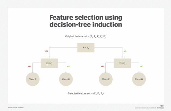
The non-leaf node performs a test on a feature, and each leaf node represents a predicted class. The algorithm only chooses the most relevant feature at each non-leaf node. The complete tree represents the subset of most value-bearing attributes (Figure 5).

Feature extraction: Overview

• How can the number of features in a data set be reduced so that the predictive potential of such features is on par with the filtered features?
• In a bid to develop a simple model, dropping features from a data set can potentially lead to a less effective model with poor accuracy.
• Rather than filtering out the features, the majority or all features are kept, and the predictive potential of all features is captured by deriving new features.
• A limited number of new features is generated by subjecting the data set to feature extraction techniques, such as principal component analysis (PCA) and singular value decomposition (SVD).

Problem

When a data set comprises a number of features, one way to reduce the number of features is to apply the feature selection pattern. This works when the filtered-out features do not actually contribute to making the model any better, but instead introduce computational complexity. However, when all features contribute to the efficacy of the model, then filtering them out is not an option. Also, from a data set exploration perspective, trying to visualize more than two features at a time, such as in a scatter plot, becomes difficult (Figure 6).

Solution

Instead of being filtered out, features are subjected to a statistical technique that summarizes the complex correlation between the features into a user-defined number of features that are linearly independent. Doing so not only reduces the feature space, but also helps to reduce overfitting. It also helps with exploratory data visualization as it converts n-dimensional space to normally two-dimensional space.

In some cases, the application of this pattern can also result in the creation of new features from scratch, an activity known as feature engineering. It is widely applied in image classification tasks where distinguishing features are extracted from training image data sets in order to represent each image as a feature vector. A feature vector is a set of features and/or attributes represented as an ordered list of fixed length that describes an object. In regression, this is the set of independent variables.

Application

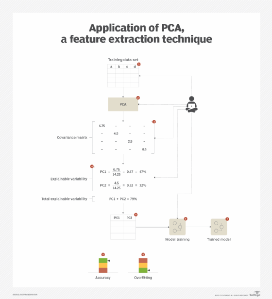
PCA is applied, which operates under the principle of removing correlational redundancy. In a data set, certain features are generally correlated in a linear manner -- in other words a straight-line relationship -- which means that such correlated features can be combined together linearly into fewer sets of features while still maintaining the predictive potential of each feature. This technique looks for combinations of features that can explain the maximum possible variation present within the feature values. In turn, this helps to make more robust models with reduced overfitting as they work equally well when they are fed varied data beyond the training data.

Based on the aforementioned explanation, the combination of features into a new feature results in a principal component. Each principal component is capable of describing a certain amount of variability in the data set. The required number of principal components or features is then chosen based on how much variability needs to be explained in the data set. For example, the top two principal components are chosen to explain 85% variability in the data set for a certain scenario.

This process involves calculating the covariance matrix of the data set. The matrix is then converted into a set of corresponding principal component values matrix, where the diagonal (top-left to bottom-right) represents the eigenvalues sorted in descending order (Figure 7). Each eigenvalue represents the factor of total variability that it can explain. Principal components are then chosen until their cumulative variability falls within the target variability that needs to be explained.

What's next?

In the next article, we will explore the feature selection and feature extraction data reduction patterns.