What is a MAC address and how do I find it?

What is a MAC address (media access control address)?
A MAC address (media access control address) is a 12-digit hexadecimal number assigned to each device connected to the network. Primarily specified as a unique identifier during device manufacturing, the MAC address is often found on a device's network interface card (NIC). A MAC address is required when trying to locate a device or when performing diagnostics on a network device.
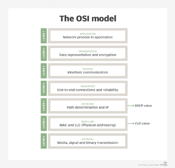
The MAC address belongs to the data link layer of the Open Systems Interconnection (OSI) model, which encapsulates the MAC address of the source and destination in the header of each data frame to ensure node-to-node communication.
Each network interface in a device is assigned a unique MAC address, so it's possible for a device to have more than one MAC address. For example, if a laptop has both an Ethernet cable port and built-in Wi-Fi, there will be two MAC addresses shown in the system configuration.
How to find the MAC address
A MAC address is often required when configuring a network router for device filtering or during network troubleshooting.
While logged in to a device, a user can typically find a MAC address in the system settings, general information or network settings and status of the device. Commonly, the MAC address is affixed to the bottom of a device on a printed label. Sometimes, manufacturers identify a MAC address by other names, such as physical address, hardware ID, wireless ID or Wi-Fi address.
The following steps can be performed to find the MAC address on different devices.
Windows
For Windows-based machines, there are two ways to find the MAC address.
Method 1: Using the command prompt
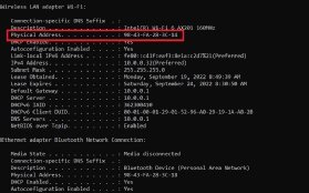
- Type cmd or command prompt in the search box of the taskbar. For older versions of Windows, right-click on the Start button, and select command prompt from the menu.
- Once inside the command prompt, type ipconfig/all, and hit Enter. This displays the network.
- Scroll down to the network adapter, and look for a value description of the Physical Address field, which is the MAC address of the device.
Method 2: Without using the command prompt
- Search and click on View network status and tasks in the taskbar, or search and navigate to Control Panel > Network and Internet > Network and Sharing Center.
- Right-click the network device whose MAC address needs to be viewed, and click on Properties.
- Look for the MAC address listed there.
Mac
- Click on the Apple icon in the top-left corner of the screen, and select System Preferences.
- Select Network.
- Select from the list the interface that needs to be used, and click on Advanced.
- Click on the Hardware tab, and find the listed MAC address.
Linux
- Log in as a superuser or with appropriate permissions.
- Open a terminal or console window.
- Type ifconfig.
- The MAC address is listed as HWaddr in a format similar to 12:34:56:78:AB.
iPhone
- Go to the Settings app.
- Select General, and click on About.
- The wireless MAC address is listed next to the Wi-Fi Address.
Android
The specific instructions for finding the MAC address of an Android device might vary by manufacturer, but the following are general steps:
- Open the Settings app.
- Select About Phone/Tablet > Status.
- The MAC address appears under Wi-Fi MAC address.
PlayStation
For PlayStation 3
- Access the PlayStation 3 main menu, and select Settings > System Settings > System Information.
- The wireless and wired MAC address should be listed on the screen.
For PlayStation 4
- Go to the PlayStation 4 main menu, and select Settings > System > System Information.
- The wired address appears next to MAC Address (LAN Cable). The wireless MAC address appears next to MAC Address (Wi-Fi).
For PlayStation 5
- From the home screen, select the settings or the gear icon in the upper right.
- Select System.
- Select Console Information.
- The MAC address (Wi-Fi) displays at the bottom of the list.
Xbox
For Xbox 360
- Access the Xbox 360 main menu, and go to My Xbox > System Settings > Network Settings > Configure Network.
- Select the Additional Settings tab and then Alternate Mac Address.
- Find the wired and wireless MAC addresses at the bottom of this screen.
For Xbox One
Use the following directions if Xbox One has been previously set up:
- From the Xbox One home screen, select Settings.
- Under the Console tab, select Network.
- Click Advanced Settings to access the wired and wireless MAC addresses.
Types of MAC addresses
There are three types of MAC addresses:
- Unicast MAC address. A unicast address is attached to a specific NIC on the local network. Therefore, this address is only used when a frame is sent from a single transmitting device to a single destination device.
- Multicast MAC address. A source device can transmit a data frame to multiple devices by using a Multicast A multicast group IP address is assigned to devices belonging to the multicast group.
- Broadcast MAC address. This address represents every device on a given network. The purpose of a broadcast domain is to enable a source device to send data to every device on the network by using the broadcast address as the destination's MAC address.
What is the difference between a MAC address vs. IP address?
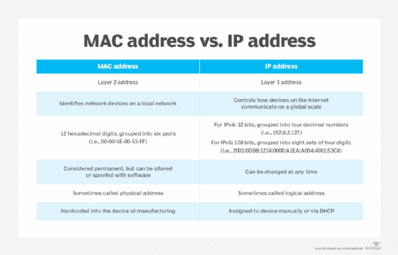
Both MAC addresses and IP addresses serve the same purpose, which is to identify a device on a network. While the MAC address identifies the physical address of a device on the same local network, the IP address identifies the device globally or through its internet address.
The following list highlights the key differences between a MAC address and an IP address.
MAC address
- is a unique hardware identifier that recognizes devices on a local scale;
- is hardcoded into the device during manufacturing;
- is sometimes called a physical address;
- can be used by a device for sending data to all devices on the same network through the broadcast MAC address;
- resides at Layer 2 of the OSI or TCP/IP reference model; and
- is permanent and unchangeable.
IP address
- helps identify a network connection;
- is assigned by the network administrator or internet service provider;
- describes how the devices on the internet communicate on a global scale;
- can be used for broadcasting or multicasting;
- resides at Layer 3, or the network layer, of the TCP/IP or OSI model;
- can be changed at any time;
- is sometimes referred to as the logical address; and
- is assigned to devices through software configurations.
Despite an organization's best efforts to keep networks running seamlessly, network issues can sometimes arise. Here's a look at common network issues and tips to troubleshoot them.