
Getty Images/iStockphoto
3 ways to evaluate and improve machine learning models
Training performance evaluation, prediction performance evaluation and baseline modeling can refine machine learning models. Learn how they work together to improve predictions.
This article is excerpted from the course "Fundamental Machine Learning," part of the Machine Learning Specialist certification program from Arcitura Education. It is the twelfth part of the 13-part series, "Using machine learning algorithms, practices and patterns."
This article provides a set of machine learning techniques dedicated to measuring the effectiveness of trained models. These model-evaluation techniques are crucial in machine learning model development: Their application helps to determine how well a model performs. As explained in Part 4, these techniques are documented in a standard pattern profile format.
Training performance evaluation: Overview
- Requirement: How can confidence be established in the efficacy of a machine learning model at training time?
- Problem: A trained machine learning model may make predictions that are randomly correct or incorrect, or may make more incorrect predictions than correct ones. Producing such a model can seriously jeopardize the effectiveness and reliability of a system. Or: Different models can be developed to solve particular categories of machine learning problems. However, not knowing which model works best may lead to choosing a not-so-optimum model for the production system with the further consequence of below-par system performance.
- Solution: The model's performance is quantified via established model evaluation techniques that make it possible to estimate the performance of a single model or to compare different models.
- Application: Based on the type of machine learning problem, classification, clustering and regression, various statistics and visualizations are generated including accuracy, confusion matrix, receiver operating characteristic (ROC) curve, cluster distortion, and means squared error (MSE).
Training performance evaluation: Explained
Problem
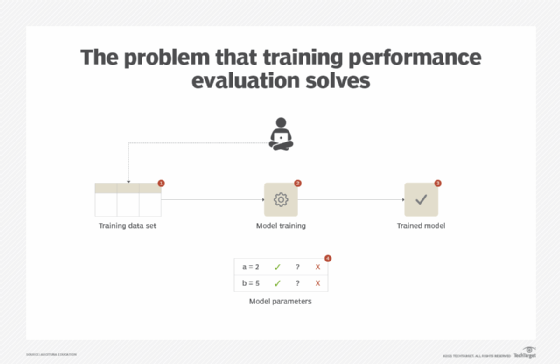
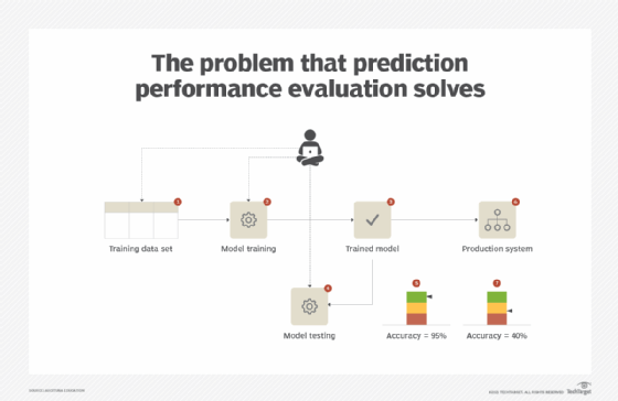
When solving machine learning problems, simply training a model based on a problem-specific training machine learning algorithm does not guarantee either that the resulting model fully captures the underlying concept hidden in the training data or that the optimum parameter values were chosen for model training. Failing to test a model's performance means an underperforming model could be deployed on the production system, resulting in incorrect predictions. Choosing one model from the many available options based on intuition alone is risky. (See Figure 1.)
Solution
By generating different metrics, the efficacy of the model can be assessed. Use of these metrics reveals how well the model fits the data on which it was trained. Through empirical evidence, the model can be improved repeatedly or different models can be compared to pick the most effective one.
Application
The machine learning software package used for model training normally provides a score or evaluate function to generate various model evaluation metrics. For regression, this includes mean squared error (MSE) and R squared (Figure 2).
Classification metrics include the following:
- Accuracy is the proportion of correctly identified instances out of all identified instances.
- Error rate, also known as the misclassification rate, is the proportion of incorrectly identified instances out of all identified instances.
- Sensitivity, also known as the true positive rate (TPR), is the probability of getting a true positive.
- Specificity, also known as the true negative rate (TNR), is the probability of getting a true negative.
- Both sensitivity and specificity capture the confidence with which a classifier makes predictions.
- Recall is the same as sensitivity: the proportion of correctly classified retrieved documents out of the set of all documents belonging to the class of interest.
- Precision is the proportion of correctly classified retrieved documents out of the set of all retrieved documents.
- F-score, also called F-measure and F1 score, takes both precision and recall into consideration in order to arrive at a single measure.
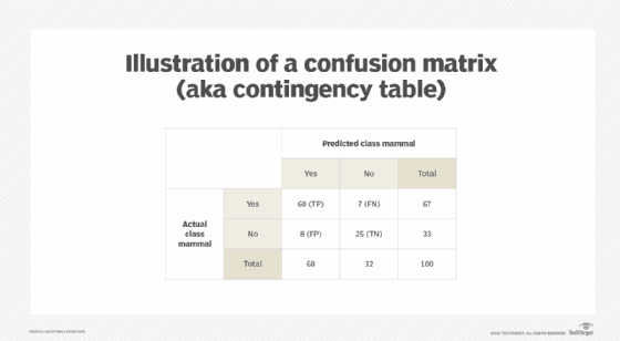
- The confusion matrix, also known as a contingency table, is a cross-tabulation that shows a summary of the predicted class values against the actual class values. Columns in a confusion matrix contain the number of instances belonging to the predicted classes, and rows contain the number of instances belonging to the actual classes.
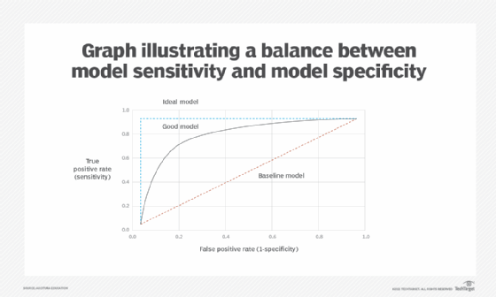
A receiver operating characteristic (ROC) curve is a visualization evaluation technique used to compare the performance of the same model or different models with different variations of the model generally obtained by trying out different variations of the model parameters. The X-axis plots the false positive rate (FPR), same as 1-specificity, while the Y-axis plots the TPR, same as sensitivity, obtained from different training runs of a model. The graph helps to find the combination of model parameters that result in a balance between sensitivity and specificity of a model. On the graph, this is the point where the curve starts to plateau with X-axis and the gain in TPR decreases but gain in FPR increases (Figure 3).
With clustering, a cluster's degree of homogeneity can be measured by calculating the cluster's distortion. A cluster's distortion can be calculated by taking the sum of squared distances between all data points and its centroid. The lower the distortion, the higher the homogeneity and vice versa.
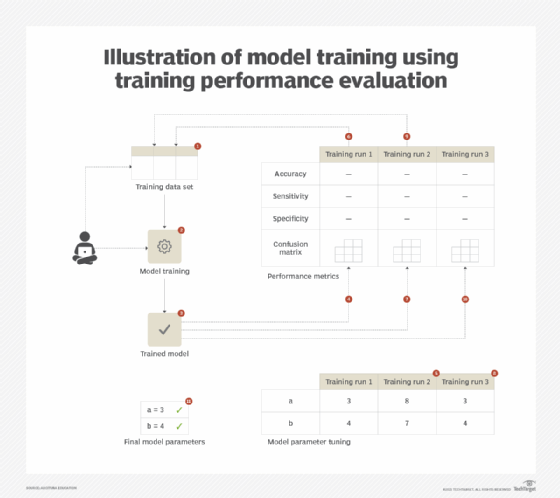
The training performance evaluation and prediction performance evaluation patterns are normally applied together to be able to evaluate model performance on unseen data. The application of this pattern can further benefit when applied together with the baseline modeling pattern. With a reference model available, different models can then easily be compared against each other as well as against the minimum acceptable performance (Figure 4).
Prediction performance evaluation: Overview
Requirement: How can confidence be established that a model's performance will not drop when it is produced and remain at par with training time performance?
Problem: A model's performance, as reported during training time, may suggest a high performing model. However, when deployed in a production environment, the same model may not perform as expected by training time performance metrics.
Solution: Rather than training the model on the entire available data set, some parts of the data set are held back to be used for evaluating the model before deploying it in a production environment.
Application: Techniques such as hold-out and cross-validation are applied to divide the available data set into subsets so that there is always one subset of data that the model has not seen before that can be used to evaluate the model's performance on unseen data, thereby simulating production environment data.
Prediction performance evaluation: Explained
Problem
A classifier that is trained and evaluated using the same data set will normally report a very high accuracy, purely due to the fact that the model has seen the same data before and may have memorized the target label of each instance. This situation leads to model Overfitting, such that the model seems to be highly effective when tested with the training data but becomes ineffective -- making incorrect predictions most of the time -- when exposed to unseen data. Solving this problem requires knowing the true efficacy of a trained model (Figure 5).
Solution
Instead of using the entire data set for training and subsequent evaluation, a small portion of the data set is kept aside. Training is performed on the rest of the data set, while the data set kept aside mimics unseen data. As such, evaluating performance on the data set provides a more realistic measure of how the model will perform when deployed in a production environment, which helps to avoid overfitting and keep the model simple. (Overfitting leads to a complex model that has captured each and every aspect of the training data, including the noise.)
Application
There are two primary techniques for estimating the future performance of a classifier:
- hold-out technique
- cross-validation (CV) technique
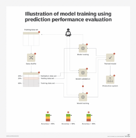
With the hold-out technique, the available data set is divided into three subsets: training, validation and test, normally with a ratio of either 60:20:20 or 50:25:25. The training data set is used to create the model; validation is used to repeatedly evaluate the model during training time with a view to select the best performing model; and the test data set is used only once to gauge the true performance of the model.
With the CV technique, also known as K-fold CV, the data set is divided into K mutually exclusive parts, or "folds." One part is withheld for model validation, while the remaining 90% of the data is used for model training. The process is then repeated K times. The results from all iterations are then averaged, which then becomes the final metric for model evaluation. K-fold CV is especially a good option if the training data set is small because the non-random split of the training data eliminates the chance of introducing a systematic error into the model when using the hold-out technique.
When applying either of these techniques, it is important to shuffle the data set before creating its subsets. Otherwise, the training and validation data sets will not be truly representative of the complete data set and will show low accuracy when evaluated using test data (Figure 6).
The training performance evaluation and prediction performance evaluation patterns are normally applied together to evaluate model performance on unseen data.
How baseline modeling aids model evaluation
How can it be assured that a trained model performs well and adds value? There may be more than one type of algorithm that can be applied to solve a particular type of machine learning problem. However, without knowing how much extra value, if at all, one model carries over others, a sub-optimal model may be selected with the further possibility of experiencing lost time and processing resources.
This problem can be solved by setting a baseline via a simple algorithm to serve as a yardstick for measuring the effectiveness of other complex models. For regression problems, for example, mean or median can be used as a baseline result while most frequent (ZeroR), stratified or uniform models can be used to generate a baseline result for classification problems.
How to set a baseline
The application of the training performance evaluation pattern provides a measure of how good a model is. However, it fails to provide a context for evaluating the model's performance; thus, the meaning of the resulting metrics may not be apparent.
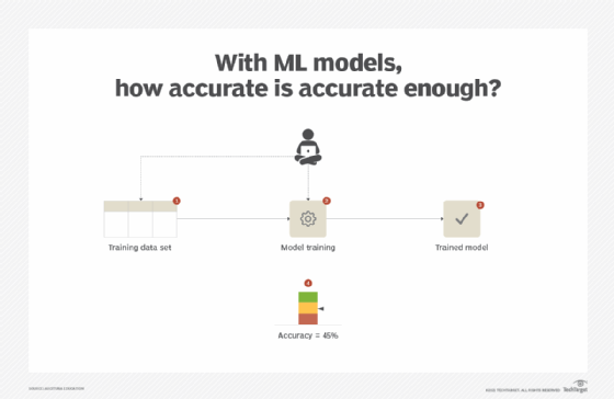
For example, an accuracy of 70% reported for a certain model is only applicable to the training data set that was used to train the model. However, what it does not report is whether 70% is good enough or whether a near accuracy can be achieved by simply making random predictions without training a model at all. (See Figure 7).
Depending on the nature of the machine learning problem, such as whether it is a regression or classification problem, an algorithm that is simple to implement is chosen before complex and processing intensive algorithms are employed. The simple algorithm is then used to establish a baseline against which other models can be compared, with a view to select only those models that provide better results.
With regression tasks, the best way to establish a baseline is to use one of the averages: mean, median or mode. The use of an average, in this case, serves well as it is the result that would normally be calculated in the absence of any machine learning model.
For classification tasks, the following options are available:
- Most frequent: The class with the most number of examples is used as the predicted class, and is also known as the ZeroR algorithm.
- Stratified: This approach considers the proportion of the classes and makes random predictions.
- Uniform: This approach gives each class an equal chance of being predicted at random.
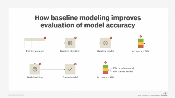
Once the baseline result has been established, other models are trained and compared against the baseline via the application of the training performance evaluation pattern.
The baseline modeling pattern is normally applied together with the training performance evaluation and prediction performance evaluation patterns. This allows evaluation of other complex models' performance on unseen data via evaluation metrics. (See Figure 8.)
What's next
The next article covers model optimization techniques, including the ensemble learning and frequent model retraining patterns.
View the full series
This lesson is one in a 13-part series on using machine learning algorithms, practices and patterns. Click the titles below to read the other available lessons.
Lesson 1: Introduction to using machine learning
Lesson 2: The "supervised" approach to machine learning
Lesson 3: Unsupervised machine learning: Dealing with unknown data
Lesson 6: How feature selection, extraction improve ML predictions
Lesson 7: 2 data-wrangling techniques for better machine learning
Lesson 8: Wrangling data with feature discretization, standardization
Lesson 9: 2 supervised learning techniques that aid value predictions
Lesson 10: Discover 2 unsupervised techniques that help categorize data
Lesson 11: ML model optimization with ensemble learning, retraining
Lesson 12
Lesson 13: Model optimization methods to cut latency, adapt to new data