CNN vs. RNN: How are they different?
Convolutional and recurrent neural networks have distinct but complementary capabilities and use cases. Compare each model architecture's strengths and weaknesses in this primer.
To set realistic expectations for AI without missing opportunities, it's important to understand both the capabilities and limitations of different model types.
Two categories of algorithms that have propelled the field of AI forward are convolutional neural networks (CNNs) and recurrent neural networks (RNNs). Compare how CNNs and RNNs work to understand their strengths and weaknesses, including where they can complement each other.
The main differences between CNNs and RNNs include the following:
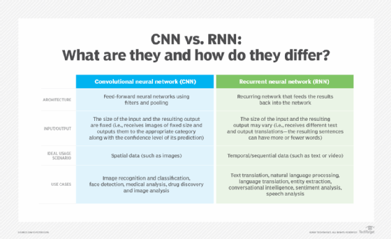
- CNNs are commonly used to solve problems involving spatial data, such as images. RNNs are better suited to analyzing temporal and sequential data, such as text or videos.
- CNNs and RNNs have different architectures. CNNs are feedforward neural networks that use filters and pooling layers, whereas RNNs feed results back into the network.
- In CNNs, the size of the input and the resulting output are fixed. A CNN receives images of fixed size and outputs a predicted class label for each image along with a confidence level. In RNNs, the size of the input and the resulting output can vary.
- Common use cases for CNNs include facial recognition, medical analysis and image classification. Common use cases for RNNs include machine translation, natural language processing, sentiment analysis and speech analysis.
ANNs and the history of neural networks
The neural network was widely recognized at the time of its invention as a major breakthrough in the field. Taking inspiration from the interconnected networks of neurons in the human brain, the architecture introduced an algorithm that enabled computers to fine-tune their decision-making -- in other words, to "learn."
An artificial neural network (ANN) consists of many perceptrons. In its simplest form, a perceptron is a function that takes two inputs, multiplies them by two random weights, adds them together with a bias value, passes the results through an activation function and prints the results. The weights and bias values, which are adjustable, define the outcome of the perceptron given two specific input values.
Combining perceptrons enabled researchers to build multilayered networks with adjustable variables that could take on a wide range of complex tasks. A mechanism called backpropagation is used to address the challenge of selecting the ideal numbers for weights and bias values.
In backpropagation, the ANN is given an input, and the result is compared with the expected output. The difference between the desired and actual output is then fed back into the neural network via a mathematical calculation that determines how to adjust each perceptron to achieve the desired result. This procedure is repeated until a satisfactory level of accuracy is reached.
This type of ANN works well for simple statistical forecasting, such as predicting a person's favorite football team given their age, gender and geographical location. But using AI for more difficult tasks, such as image recognition, requires a more complex neural network architecture.
Convolutional neural networks
Computers interpret images as sets of color values distributed over a certain width and height. Thus, what humans see as shapes and objects on a computer screen appear as arrays of numbers to the machine.
CNNs make sense of this data through mechanisms called filters: small matrices of weights tuned to detect certain features in an image, such as colors, edges or textures. In the first layers of a CNN, known as convolutional layers, a filter is slid -- or convolved -- over the input, scanning for matches between the input and the filter pattern. This results in a new matrix indicating areas where the feature of interest was detected, known as a feature map.
In the next stage of the CNN, known as the pooling layer, these feature maps are cut down using a filter that identifies the maximum or average value in various regions of the image. Reducing the dimensions of the feature maps greatly decreases the size of the data representations, making the neural network much faster.
Finally, the resulting information is fed into the CNN's fully connected layer. This layer of the network takes into account all the features extracted in the convolutional and pooling layers, enabling the model to categorize new input images into various classes.
In a CNN, the series of filters effectively builds a network that understands more and more of the image with every passing layer. The filters in the initial layers detect low-level features, such as edges. In deeper layers, the filters begin to recognize more complex patterns, such as shapes and textures. Ultimately, this results in a model capable of recognizing entire objects, regardless of their location or orientation in the image.
Bias in artificial neurons
In both artificial and biological networks, when neurons process the input they receive, they decide whether the output should be passed on to the next layer as input. The decision of whether to send information on is called bias, and it's determined by an activation function built into the system. For example, an artificial neuron can only pass an output signal on to the next layer if its inputs -- which are actually voltages -- sum to a value above some particular threshold.
Recurrent neural networks
CNNs are great at recognizing objects, animals and people, but what if we want to understand what is happening in a picture?
Consider a picture of a ball in the air. Determining whether the ball is rising or falling would require more context than a single picture -- for example, a video whose sequence could clarify whether the ball is going up or down.
This, in turn, would require the neural network to "remember" previously encountered information and factor that into future calculations. And the problem of remembering goes beyond videos: For example, many natural language understanding algorithms typically deal only with text, but need to recall information such as the topic of a discussion or previous words in a sentence.
RNNs were designed to tackle exactly this problem. RNNs can process sequential data, such as text or video, using loops that can recall and detect patterns in those sequences. The units containing these feedback loops are called recurrent cells and enable the network to retain information over time.
When the RNN receives input, the recurrent cells combine the new data with the information received in prior steps, using that previously received input to inform their analysis of the new data. The recurrent cells then update their internal states in response to the new input, enabling the RNN to identify relationships and patterns.
To illustrate, imagine that you want to translate the sentence "What date is it?" In an RNN, the algorithm feeds each word separately into the neural network. By the time the model arrives at the word it, its output is already influenced by the word What.
RNNs do have a problem, however. In basic RNNs, words that are fed into the network later tend to have a greater influence than earlier words, causing a form of memory loss over the course of a sequence. In the previous example, the words is it have a greater influence than the more meaningful word date. Newer algorithms such as long short-term memory networks address this issue by using recurrent cells designed to preserve information over longer sequences.

CNNs vs. RNNs: Strengths and weaknesses
CNNs are well suited for working with images and video, although they can also handle audio, spatial and textual data. Thus, CNNs are primarily used in computer vision and image processing tasks, such as object classification, image recognition and pattern recognition. Example use cases for CNNs include facial recognition, object detection for autonomous vehicles and anomaly identification in medical images such as X-rays.
RNNs, on the other hand, excel at working with sequential data thanks to their ability to develop contextual understanding of sequences. RNNs are therefore often used for speech recognition and natural language processing tasks, such as text summarization, machine translation and speech analysis. Example use cases for RNNs include generating textual captions for images, forecasting time series data such as sales or stock prices, and analyzing user sentiment in social media posts.
For some tasks, one option is clearly the better fit. For example, CNNs typically aren't well suited for the types of predictive text tasks where RNNs excel. Trying to use a CNN's spatial modeling capabilities to capture sequential text data would require unnecessary effort and memory; it would be much simpler and more efficient to use an RNN.
However, in other cases, the two types of models can complement each other. Combining CNNs' spatial processing and feature extraction abilities with RNNs' sequence modeling and context recall can yield powerful systems that take advantage of each algorithm's strengths.
For example, a CNN and an RNN could be used together in a video captioning application, with the CNN extracting features from video frames and the RNN using those features to write captions. Similarly, in weather forecasting, a CNN could identify patterns in maps of meteorological data, which an RNN could then use in conjunction with time series data to make weather predictions.
Dig deeper into the expanding universe of neural networks
CNNs and RNNs are just two of the most popular categories of neural network architectures. There are dozens of other approaches, and previously obscure types of models are seeing significant growth today.
Transformers, like RNNs, are a type of neural network architecture well suited to processing sequential text data. However, transformers address RNNs' limitations through a technique called attention mechanisms, which enables the model to focus on the most relevant portions of input data. This means transformers can capture relationships across longer sequences, making them a powerful tool for building large language models such as ChatGPT.
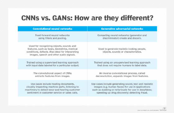
Generative adversarial networks (GANs) combine two competing neural networks: a generator and a discriminator. The generator creates synthetic data that attempts to mimic the real input as closely as possible, while the discriminator tries to detect whether data is real or produced by the generator. GANs are used in generative AI applications to create high-quality synthetic data, such as images and video.

Autoencoders are another type of neural network that is becoming the tool of choice for dimensionality reduction, image compression and data encoding. Similar to GANs, autoencoders consist of two models: an encoder, which compresses input data into a code, and a decoder, which attempts to reconstruct the input data from the generated code. The autoencoder's goal is to improve its performance over time by minimizing the difference between the original input and the decoder's reconstruction.
In addition, researchers are finding ways to automatically create new, highly optimized neural networks on the fly using neural architecture search. This technique starts with a wide range of potential architecture configurations and network components for a particular problem. The search algorithm then iteratively tries out different architectures and analyzes the results, aiming to find the optimal combination.
In this way, neural architecture search improves efficiency by helping model developers automate the process of designing customized neural networks for specific tasks. Examples of automated machine learning include Google AutoML, IBM Watson Studio and the open source library AutoKeras.
Researchers can also use ensemble modeling techniques to combine multiple neural networks with the same or different architectures. The resulting ensemble model can often achieve better performance than any of the individual models, but identifying the best combination involves comparing many possibilities.
To address this issue, researchers have developed techniques for comparing the performance and accuracy of neural network architectures, enabling them to more efficiently sift through the many options available for a given task. Creative applications of statistical techniques such as bootstrapping and cluster analysis can help researchers compare the relative performance of different neural network architectures.
Editor's note: David Petersson originally wrote this article, and Lev Craig updated and expanded it. George Lawton also contributed to this story.


