What is a perceptron?
A perceptron is a simple model of a biological neuron used in an artificial neural network. Frank Rosenblatt introduced the concept in 1957, when he demonstrated how it could be a building block in a single-layer neural network. The perceptron is considered one of the earliest algorithms created for the supervised learning of binary classifiers.
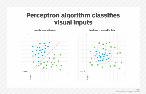
The perceptron algorithm was designed to classify visual inputs, grouping them into one of two categories. The algorithm assumes the data is linearly separable, that is, it can be naturally separated into two distinct categories. This concept can be visualized as a two-dimensional plane with two sets of data points. If those data sets can be separated by a straight line, they are said to be linearly separable. Otherwise, they're nonlinearly separable, as shown in Figure 1.

Classification is an important part of machine learning and image processing. Machine learning algorithms use different methods to find and categorize data set patterns. One of those methods is the perceptron algorithm. It performs binary classification by finding the linear separation between the data points received through the perceptron's input.
How does the perceptron work?
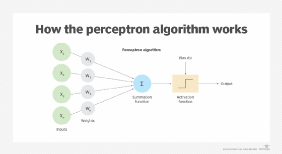
The perceptron is an artificial neuron that attempts to approximate a biological neuron. The perceptron takes one or more weighted inputs and returns a single binary output, either 1 or 0. Figure 2 shows the perceptron algorithm, in which x is the input value, w is the input's weight, and b is the specified bias (threshold).

The perceptron algorithm can be represented in various ways, often using different naming conventions, but the basic concepts are the same. The perceptron is composed of these components:
- Inputs. The perceptron receives data from one or more inputs. Each input has a numerical value that represents a data attribute.
- Weights. Each input value is assigned a numerical weight. The weight determines the input's relative strength, as it pertains to the perceptron as a whole. The input value and weight are multiplied together to come up with a weighted value for that input.
- Summation function. The function adds together the weighted values from all the inputs. For this reason, the summation function is sometimes referred to as a net input function.
- Bias (threshold). A specific numeric value is assigned to the perceptron to control the output independently of the inputs, resulting in greater flexibility.
- Activation function. The function performs a calculation on the input sum and bias to determine whether to return a binary 1 or 0. The exact approach will depend on the type of function. A step function is commonly used for the activation stage, although there are multiple other types of activation functions.
- Output. The binary result of the activation function.
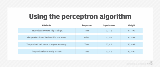
To better understand how these components work together, consider a situation in which a decision-maker wants to determine whether to purchase a product based on four attributes. Each attribute represents a binary input, in the form of true or false (1 or 0, respectively). Figure 3 lists the attributes, their input values and their weights.

In this scenario, the warranty attribute (the third one in Figure 3) is given the greatest weight and the sale attribute (the last one) is given the least. Not surprisingly, the way in which the inputs are weighted can greatly impact the outcome. The summation function adds the weighted inputs together with this formula:
z = x1w1 + x2w2 + x3w3 + x4w4
The summation function returns a single value, which the activation function then uses. To determine the input sum for the attributes, their input values and weights can be plugged into a formula:
z = x1w1 + x2w2 + x3w3 + x4w4
z = (1 x 0.7) + (0 x 0.6) + (1 x 0.8) + (1 x 0.3)
z = 0.7 + 0 + 0.8 + 0.3
z = 1.8
Here, the summation function (z) returns a value of 1.8. This value can be used in the activation function (a), along with the bias (b), which in this case has a value of 2. Activation functions use different logic to calculate the binary output value. This example applies the following logic to the summation and bias:
a = 1 if z > b else 0
The formula states that input sum must be greater than the bias for the function to return a 1. Otherwise, it will return a 0. You can apply this formula to the example above:
a = 1 if z > b else 0
a = 1 if 1.8 > 2 else 0
a = 0
The input sum does not exceed the threshold, so the perceptron returns a value of 0. This simple example demonstrates the basic concepts of how the perceptron works and applies straightforward logic.
A perceptron can also be trained via a learning algorithm. During the training period, the perceptron undergoes a period of supervised learning that uses labeled data in which the categories are already known. Based on the results of this process, the perceptron's weights and biases are then adjusted to improve the perceptron's accuracy.
A brief history of the perceptron
The artificial neuron idea predates Rosenblatt's work. In 1943, neurophysiologist Warren McCulloch and logician Walter Pitts published a seminal paper "A logical calculus of the ideas immanent in nervous activity," which provides the first mathematical model of a neural network. Their artificial neuron --dubbed the McCulloch-Pitts (MCP) neuron -- receives binary inputs and produces a binary output.

When developing the perceptron, Rosenblatt built on the concepts of the MCP neuron, but he enhanced the model to increase its flexibility. He worked on the perceptron in 1957 at Cornell Aeronautical Laboratory, where he received funding from the United States Office of Naval Research. Rosenblatt first ran the algorithm on an IBM 704 computer that weighed five tons and filled an entire room. The project represented the first step toward a machine implementation for image recognition.
The following year, Rosenblatt and his collogues built their own machine: the Mark I Perceptron. The computer contained an array of 400 photocells connected to perceptrons. The perceptron weights were recorded in potentiometers, as adjusted by electric motors. The Mark I Perceptron was one of the first artificial neural networks ever created. It now resides at the National Museum of American History, which is part of the Smithsonian Institute.
When the perceptron was introduced, many believed it represented a significant milestone in the push toward AI. However, the technical limitations of the perceptron soon became apparent because single-layer perceptrons can group data only if it is linearly separable. Later, data scientists discovered that by using multilayered perceptrons, they could classify nonlinearly separable data, allowing them to solve problems that single-layer algorithms could not.
Training neural nets to mirror the human brain enables deep learning models to apply learning to data they've never seen before. Learn how neural network training methods are modeled after the human brain. Also, explore how supervised, unsupervised, semisupervised and reinforcement learning compare to each other.
