25 machine learning interview questions with answers

Theory

1. What is the difference between supervised and unsupervised machine learning?

The main difference between supervised learning and unsupervised learning is the type of training data used. Supervised machine learning algorithms use labeled data, whereas unsupervised learning algorithms train on unlabeled data.

Labeled data contains predefined variables that guide the algorithm in learning -- it knows to some degree what it is looking for. Unlabeled data does not have predefined variables or features, so the algorithm scans the data set for any meaningful connection. Basically, the supervised algorithm learns with the help of a teacher, or supervisor, and the unsupervised algorithm learns alone. Supervised algorithms can generally produce results with a high degree of confidence but take a lot of manual effort in the process of labeling the training data. Unsupervised algorithms may be less accurate but can also be implemented with less initial work.

Semisupervised learning is a combination of both methods in which unsupervised learning algorithms generate the labels that are fed to supervised learning algorithms. In this method, there is some human involvement in augmenting the labels that the unsupervised algorithm initially generates.

Which method to use depends on the results you are trying to produce and the data you have available. Certain types of data are easier to label than other types.

Together, supervised learning, unsupervised learning, semisupervised learning and reinforcement learning make up the four main types of machine learning algorithms.

2. What is the relationship between variance and bias?

Machine learning bias is when an algorithm produces prejudiced results because of erroneous assumptions made during the ML process. It is error due to oversimplification.

Variance is error due to overcomplexity in a learning algorithm, which causes too much noise in the test data.

The relationship between these two terms is sometimes framed as the "bias-variance dilemma" or the "bias-variance tradeoff" and is considered a main problem in supervised learning models, partially due to the fact that unconscious human biases enter the ML process when humans label the training data. Basically, the lower the bias in an algorithm, the higher the variance, and vice versa. An algorithm with high variance but low bias may represent the training data set well but may also overfit to unrepresentative data. An algorithm with high levels of bias may underfit its training data and fail to capture important characteristics of the training set because it is oversimplifying.

The way to reduce bias is to make a model more complex and add variables (features), and to do the opposite to reduce variance. A method known as the bias-variance decomposition is used to evaluate an algorithm's expected generalization error. Another method -- known as the kernel trick -- can be used to make complex data sets more manageable.

In statistical theory, if you were to take a poll of people (for instance, leading up to an election) you are sampling a portion of the overall population. One of the first issues that you face in performing such a poll is whether the sample represents the overall population. For instance, if a poll is conducted using land-line phones, this may exclude a significant percentage of the population who only use cell phones, and if land-line phones are found to correlate with one party over another, this could skew the results systematically in one direction or another. This is known as bias.

At the time of that poll, a person could be uncertain about which candidate they are going to choose and they could change their mind later. Put another way, the signal from that particular person is weak, and if that's true of the overall electorate, then the uncertainty about the poll's accuracy is likely higher. This uncertainty is known as variance or variability.

Machine learning data faces the same issues. When the sample set (the learning set) comes from a biased source, meaning that sample set was not representative, then you will have a strong signal that's likely to deviate from reality. You can compensate for this by tweaking the model to weaken the bias, but you are still very much beholden to the quality of the inbound data.

When you have a high degree of variance, and hence low signal strength, this usually means that the margin of error is likely to be higher. Increasing the overall sample size can help, as can attempting to boost the signal by adding correlative factors (e.g., socioeconomic status, gender, geographical location or ethnicity) that may better give an indication of how they are likely to vote.

Note that bias and variance influence one another. Bias can be thought of as the deviance of the sample mean (the average of the sample in all dimensions) as compared to the population mean. In an ideal world, there should be no difference between these two means, but reality is usually not that forgiving, so typically data scientists should assume that there is likely a normal or bell curve that determines the probability that the sample mean is likely to be off by a certain amount. The variance determines how wide the bell curve is. Both of these factors ultimately determine the margin of error, though bias generally cannot be measured directly.

3. What is the difference between probability and likelihood?

Roll a six-sided dice. The chance of one number coming up (say a 3) is one in six (assuming a fair dice). If you graphed this distribution based upon frequency of occurrence, the graph will be pretty monotonous -- a horizontal line of unit height. This is called a uniform distribution. If you paint one dice blue and the other red, then roll them together, the distribution for each color will be the same. The dice are considered independent in that they do not affect one another.

However, when you roll those two die together and add their sum, the sum depends equally on each, so that you are now measuring the number of combinations that will add up this distribution. This distribution will look like a triangle, (2:1,3:2,4:3,5:4,6:5,7:6,8:5,9:4,10:3,11:2,12:1), where the first number in each pair is the sum, and the second is the number of combinations. With three dice, the distribution begins to approach a bell curve (or more properly a binomial distribution). If you divide the total number of states, in this case 6x6 (36) and 6x6x6 (216) respectively, you get what's called a normalized distribution: The total of each fraction of the whole will be equal to 1.

As the number of die (each independent but of the same number of faces) becomes larger and larger, this eventually creates a continuous curve or envelope called a Gaussian distribution. Gaussian distributions are significant because they pop up when you are measuring a certain property that may have many independent states.

It also turns out that if you take such a distribution and measure the area underneath it (through calculus), the highest point in the curve (on the y axis) represents even probability -- 50% of the population will be on one side of the symmetric relationship, the other 50% will be on the other, with the probability of a given sample being proportional to its standard deviation from the mean, where a standard deviation is essentially the square root of the sum of the squares of the differences of the variances from the mean.

This means that if you know the mean height of an adult male (about 5'10") and you can show that 67% of the population (1 standard deviation past the mean) are 6'3" or under, then you can use it to predict the number of men who will be 6'9" or 4'10". This number is, for a given distribution, the probability that a given sample will be of that value.

Note also that if the distribution is not quite symmetric (perhaps in the die example that someone weights all die to preferentially show 6), then the skew of the distribution curve can be one way to measure the bias in a given sample.

Likelihood is a related concept but is not quite the same thing. A good example of understanding likelihood (at least to American readers) is the question of "if a given candidate wins a certain state, such as Texas or California, in the election, what is the likelihood that they will become president?" This is a surprisingly complex problem, because typically, states are very seldom independent races. Instead, the chances are good that if you win California, then you will likely also win Washington, Oregon, Hawaii, New York, Massachusetts and several others. Similarly, winning Texas will bring with it a different constellation of states.

In other words, unlike in the first case where your variables are independent (there is no correlation or anti-correlation), here the variables are typically interconnected. Mathematicians refer to the first as saying that the variables are orthogonal -- no one variable contributes to the value of another variable -- while in the second case they are not. Orthogonal variables are usually easy to decompose into independent problems (or dimensions) while nonorthogonal variables almost always have hidden variables and dependencies.

So likelihoods can usually be stated as, "Given event A, what is the likelihood that event B will occur if event B depends upon event A?" This is the foundation for Bayesian analysis, based upon Bayes Theorem. Additionally, Bayes Theorem in term has dependency upon Markov Chains (or Markov Graphs), which basically perform complex analysis by determining the values of associated nodes in a graph as weighted probabilities. Such solutions can be solved using statistical algorithms, weighting coefficients in neural nets, or through the use of graph theory. If the terms probability and given are contained in the same problem, it's usually a pretty good likelihood that Bayes Theorem is involved.

4. What is the curse of dimensionality and how would you respond to it?

Most modern data science and machine learning makes use of the term features instead of variables, but the idea is much the same. Most statistical problems come down to determining the number of variables (features) that are relevant to understanding the problem, then converting the values into numeric ranges between zero and one (or occasionally -1 and 1). This is the process of normalization. The process of optimizing variables, normalizing them, and determining which are relevant is known as feature engineering.

This makes a bit more sense when talking about ranges from -1 to 1 (although most algorithms use 0 to 1), but for purposes of illustration, let us use the larger range. What this means is that if you define the height of a person, then a height of 1 indicates the tallest people in that range, while a height of -1 correlates to the shortest (or anti-correlates to the longest), and 0 (the average) then becomes the midpoint. These are typically known as normalized vectors.

In an ideal world (mathematically), each vector is treated as being orthogonal to other vectors. If one vector goes from left to right, a second vector from bottom to top, and a third goes from it to out. These are called dimensions, though they're not necessarily the same thing as the three spatial dimensions that we are aware of. They may represent things like height, age and political orientation. This means that you can represent this cluster of traits -- or features -- as a point in this three-dimensional space for a given individual, or a zero-based vector emanating as a deviation from the mean.

Mathematicians are used to thinking in more than three dimensions. A four-dimensional vector is simply another orthogonal value to the other three. We can't visualize it directly in three dimensions, but we can create shadows (or projections) of all four of these vectors upon a plane or three-dimensional space, typically using other attributes such as color, size or texture of the represented point. Five dimensions are harder to visualize this way, but abstractly the idea is the same. In a machine learning context, it is possible to have dozens, hundreds, or even millions of such features. A computer simply treats these as arrays (or sequences) of the corresponding number of dimensions.

Typically, one of the goals of this kind of analysis is to determine clusters where similar individuals occupy the same general proximity in this "phase space." This is used heavily for classification purposes, defining neighborhoods that identify that the clustered data points identify a class. In a small number of dimensions, such clusters usually are self-evident, but as you increase the number of dimensions, there may be features that are totally opposite one another that increase the apparent distance between those points. For instance, let's say that you have a feature set that identifies characteristics that distinguish between cats and dogs.

However, one of those features is gender, which in fact may be central to the definition of the animal in question, but which places at least half of all elements clear across phase space from the other half. The clustering becomes obvious if you take that feature out, but if you don't know a priori what a given feature actually means (and you may not) then you may be hard pressed to say that male and female cats are both cats.

This is another way of saying that as you add more features, the points that represent these individuals can move so far away from one another that they can't form useful neighborhoods. The vector space is said to become sparse at that point. You have too many dimensions, which is where the term curse of dimensionality comes from.

The best thing to do in this case is to cut down the number of dimensions in your model. It may sound impressive to say that you are working on a model with a million dimensions, but most of those dimensions likely do not contribute significantly to the overall model accuracy but do have a major impact upon how long (how much data) it takes for a model to be trained. Analyses can be done on manifolds that can determine whether a given manifold (a space made from a smaller number of dimensions) provides meaningful impact to the model overall. Common methods for dimensionality reduction include principal component analysis, backward feature elimination and forward feature selection.

This is especially true in unsupervised learning systems, Sometimes, clusters form that are random noise that don't really have any significance in the model at all. In general, by reducing the number of dimensions by analysis of manifold impact, you can get down to a point where a model not only provides more meaningful data, but it does so requiring less data be processed in a shorter period of time.

5. Can you explain the difference between a discriminative and generative ML model?

Let's revisit the concept of distributions again. A distribution can the thought of as the continuous version of a frequency diagram. In taking the sum of three dice, for instance, there is a minimum value (3) and a maximum value (18) that constitute buckets. The 3 bucket has only one potential configuration (all three dice have a value of 1). The 18 bucket is the same -- in both cases the probability of rolling a 3 or an eighteen is 1/216, a shade under half of one percent. In the middle, there are also two buckets, buckets 10 and 11, that each have 36 possible configurations that will add up to 10 or 11 respectively, so the probability there 36/216 = 1/6=16.67%.

If you view each collection of buckets as a feature, then the probability associated with the bucket can be determined from the frequency distribution divided by the total number of states (or the normalized equivalent for a continuous distribution). In the case of a uniform distribution (such as rolling one red dice and comparing it with the role of another blue dice), this calculation becomes trivial -- it is (1/r)*(1/b) where r and b are the number of pips on each dice.

Suppose, however, that you and I each had a set of three dice each, yours red and mine blue. The probability that your red dice would roll a 10 and my blue dice would roll an 18 would be P(10)*P(18) = 1/6 * 1/216 = 1/1296. On the other hand, the probability of my rolling a ten and you rolling an eleven is much higher. P(10)*P(11)= 1/6 *1/6 = 1/36 (or thirty six times more likely). This is called a bivariate distribution, and is usually written as P(X,Y) where X and Y vary over their respective ranges.

When generalized to N different features, this is referred to as multivariate distributions or, more frequently, as joint distributions. At any given point in this N-dimensional feature space P(X₁,X₂,…,X_N), the associated probability will be the product of all of the independent probabilities at those respective points, what's often referred to as the probability density.

A generative machine learning model is one where the functions that determine the various coefficients of that model are determined by using the overall joint distribution of all of the features. This can be comprehensive, because each feature fully informs the overall probability, but it is also computationally expensive, as you also have to calculate the probability density across a mesh of N dimensions, which increased by the number of points in each message (say you sample across 10 points in any given dimension) to the Nth power. A model with 10 dimensions would take 10 to the 10th power calculations (about 10 gigaflops), which is quite doable (about 1 microsecond) on something like the recently announced Xbox X Series GPUs, which is capable of 13 teraflops. A model with 15 features or dimensions, though, would take 10 minutes to do the same thing, and a model with 100 dimensions would take longer than the universe is likely to be in existence.

A discriminative model, however, uses Bayesians to partition the problem domain in different ways, reducing the number of dimensions by filtering out those that don't contribute materially to the overall model. Discriminative models basically look at the differences between sets, meaning that they don't necessarily have as much information as generative models do, and so are likely to be less accurate, but they can calculate results in a much shorter period of time.

6. Can you explain the Bayes Theorem and how it's useful in ML?

So what, exactly, is a Bayesian? Joint distributions work upon the assumption that two or more distributions are independent of one another. Many times, however, that's not the case. For instance, in a human population, height and weight are definitely correlated. In general, your weight varies according to two factors -- your height and your girth, in effect, your average radius across the sagittal (top to bottom) line of your body. You may be tall and skinny or short and stout and have the same weight, but if you constrain one of those two, the other will have a linear relationship. I'm assuming, for ease of discussion, that average density remains constant, as mass = volume x density.

Now, height, girth and mass all are distributions. Bayes Theorem can be stated as follows:

P(A|B) = P(B|A) x P(A)/P(B)

Where A|B should be read as A given B. In English, this translates to the following:

The probability of A given B is the same as the probability of B given A x the probability of A divided by the probability of B.

This is not necessarily that much clearer, so again, let's think of this in terms of the example given above. The probability that you will have a certain weight given you have a specific height (how much do I weigh if I'm six feet tall) is going to be the probability that I'm going to have a certain height if I weigh 200 pounds, times the probability that I weigh 200 pounds divided by the probability that I am six feet tall.

We can determine P(A) and P(B) by surveying a population and coming up with a distribution. If you assume that each of the distributions is a Gaussian function, we can determine that the probability of you being six foot tall puts you at the 84th percentile (see this handy-dandy height calculator) and the probability that you are 200 lbs is the 58th percentile (similar handy-dandy weight calculator). This simplifies the equation down (for this one data point) to:

P(W=200|H=6.0) = P(H|W) * P(H)/P(W) = P(H|W) * .84 / .58 = 1.45 * P(H=6.0|W=200)

Now, this doesn't necessarily tell you a lot, but it tells you something important -- if you go out and sample 10,000 men for their height and weight and create a bivariate distribution, you can use this to create a table that will let you determine roughly what P(H|W) looks like. Once you have that distribution function, you can use it to determine the distribution function for P(W|H).

To carry this through, let's say that you surveyed 1,000 men, 30 of them were 200 lbs and of those 15 were 6' even. This means that P(H=6.0|W=200) = 15/30 = 0.5. Completed this equation, you could then say that:

P(W=200|H=6.0) = P(H|W) * P(W)/P(H) = 0.5 * 0.84 / 0.58 = 0.72, or 72%

The expression P(A|B) is typically known as the posterior distribution, with P(B|A) referred to as the likelihood, P(A) being called the prior distribution and P(B) being called the evidence distribution. In our sample above, P(W/H) is the model about weight given height we don't know yet but are trying to determine, P(H/W) is the model of height given weight that we do know (or at least have a pretty good idea about), P(H) is the prior knowledge and P(W) is the data.

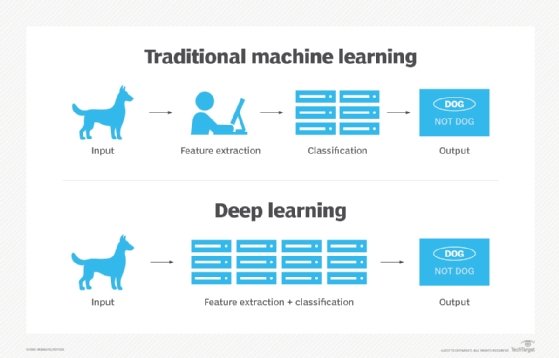
7. What is deep learning, and how does it differ from machine learning?

Deep learning is a subset of machine learning that imitates the way humans learn using neural networks, backpropagation, and various neuroscience principles to accurately model unstructured or semistructured data. Because machine learning is a broader category than deep learning, deep learning can be thought of as a machine learning algorithm that specifically uses neural nets to learn data representations.

Neural nets were first hypothesized in the late 1940s by Donald Olding Hebb as a theory of neuroplasticity. In the 1960s, Frank Rosenblatt proposed a specialized computer circuit, based upon Hebb's theories, which is now considered the first computer model of an artificial neuron. Rosenblatt's untimely death in 1971, as well as scathing criticism by Marvin Minsky and Seymour Papert, who had published their own models about neurons called perceptrons, put a significant damper on additional research in the field until the 1980s. This additional research ultimately proved that Rosenblatt's models were more correct. Even there, however, most neural nets, which involved non-linear mathematics, were simply too slow given the technology to be fully developed.

It would take another 30 years before the technology caught up with the theory, and for neural nets to gain ascendancy. Neural nets work by taking a particular programming problem (such as analyzing the shape of handwritten characters), decomposing them into specific sub-patterns, then using arrays of non-linear equations to determine the coefficients involved in those equations. This process, called backpropagation, takes an initial guess and associates weights with each coefficient to determine the strength of a particular input.

Supervised learning, in which each data instance is labeled to identify the relevant characteristics, can usually produce higher quality results, but requires the curation of source materials. Conversely, unsupervised learning looks for patterns without initial prejudice. It is not as accurate and requires a large starting set but doesn't require that curation. Recently, more complex algorithms have emerged which use systems of ongoing "rewards" and "punishments" to change the coefficients over time, which means that a given actor will appear to learn to optimize changing conditions. This is called reinforcement learning, and it is increasingly used to drive agented systems and computer games, for example.

The advantage that neural networks have over more algorithmic approaches is that they can facilitate transactions when the underlying model driving the system is unknown. The disadvantage of such systems is that it is often difficult to understand why a given model makes the decisions that it does, a process known as lack of explainability. Most recent deep learning work is now focusing on that particular problem.

8. What is ensemble learning and what are its benefits?

In weather forecasting, especially when trying to determine the likely tracks of hurricanes, it is not uncommon for different organizations to create different models working with different core assumptions but usually the same base data. Each model in turn is updated with new information in real time. These agencies then frequently publish the models they used in comparison to how the actual hurricane proceeded, so that all agencies can see what proved to be consistently predictive over several storms.

An ensemble in data science can mean several things, but usually involves the creation of models that may have the same dimensional features but have different starting conditions or underlying assumptions. These can then be combined via straightforward linear algebra principles.

9. How do ensemble models, like random forests and GBMs, differ from basic decision tree algorithms?

When we make decisions, typically, there is more to a given decision than "yes" or "no." There could be several independent factors that need to be evaluated, and the answer to one changes the response to the next. For instance, consider a case of someone buying a car. There may be two distinct factors: whether a person is young or old and their level of wealth. If these factors are unrelated, then the decision is an easy one -- it's contingent upon the level of wealth.

However, if you, as a salesperson, are trying to assess whether a person walking onto the lot will buy that car, you have likely made some observations based on experience, for example:

• If a person is under the age of 30, they will buy a car if they have a high income but won't if they have a low to medium income.
• If a person is between 30 and 60, they will buy a car if they have a medium to high income but won't if they have a low income.
• If a person is older than 60, they won't buy the car regardless.

These assumptions can be demonstrated as a decision tree.

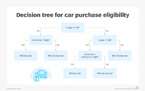
Each branch point in the tree is a conditional that reflects previous decisions. Because income is at least somewhat correlated to age, the dependent variable (income) occurs after the independent variable (age) has been ascertained. In sales-speak, you'd say that the decision tree is used to qualify the buyer -- the seller should spend less time trying to convince an unqualified buyer to spend the money because the likelihood that they will is much, much lower. The leaf nodes, on the other hand, give a particular outcome -- here, whether a person will or won't buy the care if persuaded.

The decision tree is a form of classification, with the guessing game twenty questions -- in which a person tries to guess what a thing is based upon yes or no answers -- being the archetypal example. Note that decision trees do not actually tell you the likelihood of any state, but rather, simply give you an indication that, if these conditions hold, then this is the possible outcome.

Most decision trees can be quite complex and usually incorporate a probability measure of some sort of the form, "Given this condition is true (or false), what is the probability that an action is taken?" The salesperson can assess the age of the individual directly but, until confirmed, can only guess at their income level based upon other, more subtle clues, such as the way that they dress. Trees with such probabilities at the yes-no branch points are usually referred to as Bayesian trees and form the bulk of all decision trees that aren't purely algorithmic.

A decision tree is a machine learning model -- it predicts various outcomes if specific conditions are held to be true. When you change the weights of the decision points, you are, in effect, creating a new model. Typically, a researcher tests the models by choosing different sets of starting points and weights, in order to see what the likelihoods of specific outcomes are. The set of all such models that the researcher creates is known as an ensemble.

A good example of an ensemble model is the path and intensity of a hurricane. All hurricanes start out as invests, which are areas of low pressure that form as part of turbulence in the atmosphere. Atlantic hurricanes, for instance, almost invariably start off the coast of West Africa, usually as heat and sandstorms from the Sahara deserts.

If the storms are not broken up by the mid-Atlantic wind shear, such storms gain strength if the Atlantic waters are warm enough and then follow a path up into the Caribbean Sea. Once there, their exact path may take them up into the Gulf of Mexico or across Florida; though, if they make landfall on an island, the temporary lack of moisture and heat may disorganize and weaken them. Because of this, such storms may hit as far south as Panama and as far north as New England in the United States.

Predicting the paths and intensities of such models is extraordinarily compute-intensive, and as such, different forecasting agencies usually develop their own models and compare them as part of an ensemble. To cut down on some of the complexity, a random forest approach may be used in which different potential configurations within the larger model are swapped in and out, in order to determine the model's sensitivity to change. In this case, the goal is to reduce overfitting where possible, which is easier done when parts of a model remain fairly invariant. The position of invests, for instance, tends to be restricted to a fairly narrow band along the African coast, and as such, the data is less noisy and can be modeled with a fairly high degree of confidence.

Gradient Boosting Machine (GBM), on the other hand, starts with an ensemble model but then boosts certain parameters based on the errors from previous models in the ensemble. Put another way, with GBM, previous ensembles are used to partially train the current models where they are similar enough. GBM tends to be less immediately compute-intensive -- in effect, the models are learning from previous models, as well as current data, but the likelihood of overfitting is also somewhat higher.

Random forest and GBM can be used together as predictive techniques in a process called ensemble stacking -- or, more colloquially, just stacking. In essence, the weights of random forest and GBM models are used to create a single metamodel that can give a closer approximation to the real data without overfitting. The disadvantages of such a metamodel, however, are that it is both more complex and computationally much more expensive.

10. What are overfitting and underfitting and how do you avoid each?

In data analytics, you frequently have a large number of data points coming from your data source. Your goal with that data is to generate a model, which, in this case, is a function specified as a polynomial in one or more dimensions. For example, suppose that you are tracking a stock on the stock market over a period of 30 days, as seen here.

You want to create a mathematical model that describes the behavior of that stock. Your goal is to create a polynomial of the form:

F(t) = a₀ + a₁x + a₂x² + a₃x³ + a₄x⁴ + … + a_nxⁿ + …

Each constant a_i determines the influence of the particular exponential term. A naive approach might be to include as many coefficients as possible in order to generate a curve that closely matches the data points (the red line in the chart here).

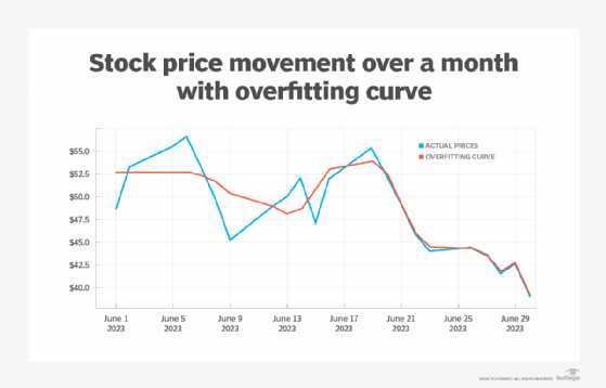
This curve closely matches the data points from about June 20 on, though it doesn't handle the larger fluctuations before then as well. However, remember that each price value only matches the movement at the end of the day and is, in effect, a sample that may hide a lot of variability.

In creating a curve that matches the data set too closely, the randomness of the data set gets captured as well, making such a curve less than ideal for determining trends. By attempting to model in this way, you are oversampling -- capturing too much of the noisy randomness of the system without getting a good indication of the broader term behavior.

On the other hand, you might also end up going in the other direction -- making your model too coarse by having too few terms defined in the set of polynomials. This can give you a smoother graph but at the expense of a higher degree of likelihood that the model doesn't capture the trends in the data at a sufficient degree of granularity. This is called undersampling (in green in the chart here).

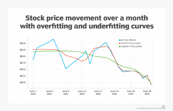
The undersampling curve roughly follows the oversampling curve, but the variations are usually too smoothed out to be meaningful.

What a good modeler is looking for is an optimal fit, something that is neither too jagged nor too smooth. The optimal fit might look something like the cyan curve in the chart below, especially towards the end of the month.

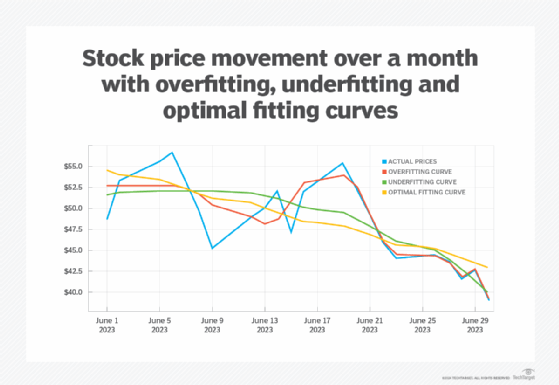
The optimal curve usually is found by creating a rolling average of values at any given point of previous data points and then using this to normalize the values of the data set. This process will likely lose some of the noise in the original sample, and of course, it will be less accurate at the start of such a curve because you're reducing the number of data points in the average. But, at the same time, it provides a more accurate trend line that doesn't require as many terms in the polynomial itself.

Note that this type of analysis is what a neural network uses to determine an optimal traversal surface, while attempting to minimize the noise in the system. There are multiple strategies for finding optimal fits, but most of them use some variation of smoothing to even out the spikes.

11. What is regularization in machine learning? And what is the difference between LASSO and Ridge regularization techniques?

To understand regularization, it's necessary to understand the role of loss functions, also known as cost functions, in machine learning. A loss function is a measure of the deviance between the predicted value determined in the model and the actual value as given in the data for that model; it plays much the same role in an ML model that standard deviation performs in traditional data analytics.

The goal of any machine learning model is to minimize the overall loss function for that model -- in other words, for a sufficient set of new data, the values predicted by the model for that data should be as close to the actual data as possible.

The problem with this is that most real-world data is fundamentally noisy -- there may be errors due to variations in sampling and reporting, changes in environmental conditions, malfunctions and assumptions that may not have been captured in the model but should have been. For instance, in political campaigns, it is not uncommon for some new news about a given candidate to cause a spike in awareness that shows up as a transient shift but, ultimately, has only a small impact on measured sentiment.

Regularization is the process of trying to account for those outliers, while, at the same time, not losing the broader trend of the data -- i.e., trying to find an optimal fit for the data, even given these outliers -- usually as part of refining the model. In general, regularization works by adding a penalty term to the model's loss function that compensates for the Z-value of the data points in question.

There are two well-established techniques for doing this: LASSO and Ridge.

LASSO is an acronym that stands for least absolute shrinkage and selection operator. The LASSO technique takes the coefficients of the loss function and then sums up the absolute values of these coefficients and combines it with a weighting factor. This approach, in effect, reduces the contribution of certain coefficients to zero, removing them from the weighting factor altogether. This is especially useful when you have a lot of features but anticipate that only a few of them contribute anything of value to the overall model. This tends to reduce the noisiness of irrelevant features, making for a better-fitting curve overall. LASSO is also known as L1 regularization.

Ridge, on the other hand, uses the squares of the coefficients, rather than their absolute values. This works better in scenarios where you have lots of features that might contribute some value to the overall model and you don't necessarily know what those features are. Ridge tends to be a little noisier than LASSO but is more accurate where you have a lot of interdependency between features in your feature set. Ridge is also known as L2 regularization.

12. What's the difference between a type I and type II error?

In analyzing data, you typically have to make a conclusion based upon the model that you create. For instance, if you have a particular vaccine, your conclusion may be that the vaccine is effective against a specific virus. However, there are, in fact, four possible states about that conclusion, depending upon your belief vs. the reality of the test:

1. You believe the virus is effective, and it is (true positive).
2. You believe the virus is effective, but it's not (false positive).
3. You do not believe the virus is effective, when it is (false negative).
4. You do not believe the virus is effective, when it's not (true negative).

The second scenario describes a false positive situation, which is also known as a type I error. False positive situations usually arise when your model classifies a given entry in the test data, as opposed to the training data, as being of a certain categorization, when, in fact, it is of a different categorization. An example of a false positive is when you take a test for having cancer and it comes back positive when you don't have it.

The third scenario describes a false negative situation, which is also known as a type II error. False negatives are similarly misclassification problems and occur when the model fails to catch that a given entry in the test data corresponds to a given categorization. An example of a false negative is when you take a test for cancer and it comes back negative when you do, in fact, have it.

False positives (type I errors) usually arise because the model's criteria for classification are too ambiguous, meaning that a given entry could be classified in more than one way and it just happened to trip the conditions that put it into the wrong bucket. This is often also caused when the data is too noisy and overfitted. The best solution there is to reexamine your model and see if there are features that have been missed, as well as to regularize your models to better compensate for that noise.

On the other hand, false negatives (type II errors) typically occur when your model is not discriminating enough or when the sampling from the data is insufficient to resolve the relevant classification criteria. Type II errors can also be thought of as sensitivity errors -- there are simply not enough samples in your data set to register. But it could also be that you need to tighten up your model by increasing the fit against the mean.

This sensitivity is often called the significance level and is described by two parameters: α (type I error) and β (type II error). Similarly, you can rephrase your conclusion as a null hypothesis (H₀), which is the stated hypothesis, and an alternative hypothesis (H₁), which is the opposite conclusion. In modern statistics, the significance parameters are often inversely correlated -- the more that you try to reduce α, the more likely you are to increase β. But this is complicated by the fact that these are both also functions of the deviation from optimal fit.

13. What are outliers? What tools and strategies would you use to identify and handle them?

Outliers are data points from a sample that, for some reason or another, do not follow the trend of the other data points. For instance, suppose that you have a network of ocean buoys that measures (samples) the temperature of water at a fixed location. The temperatures from one buoy to the next vary, potentially dramatically, but in general, the temperatures are unlikely to vary much from one sampling period to the next for any given buoy. Moreover, adjacent buoys are likely to have similar temperatures that vary in a predictable pattern.

Suppose, however, that, as you are looking at the data sets, you see one buoy in particular that sees a sudden spike or drop in temperature that seems inconsistent with both its own behavior and with the behavior of other buoys around it. The measurements from this particular buoy are inconsistent and thus are considered outliers.

You probably can't tell why the buoy's behavior has changed. It's possible that a sea lion decided to lay on the sensor, the buoy malfunctioned or a wave swamped it. It is also possible, though less likely, that the buoy is working perfectly but the environment around it is changing, indicating the start of a new trend.

This is why outliers can be problematic. Usually, the best thing that you can do in the scenario described is to continue to monitor the outlier, as well as other sensors that are in the general proximity of that buoy. If the buoy continues to send anomalous signals, then it is likely that buoy is malfunctioning and should be checked. However, if nearby buoys also begin to register the same behavior, then it is more than likely a new trend forming.

For instance, let's say that you have a sensor grid with buoys at one-mile intervals. If the temperatures indicated by the buoys over a few hours then rise again, it may indicate a passing iceberg in a shipping lane. In effect, the changes you are seeing are significant -- they are a signal that something is changing. An unexpected blip and then a sensor returning to normal, on the other hand, may well be noise in the measure, e.g., a seal sleeping on the sensor.

Most statistical analysis tools work by measuring the standard deviation of a signal away from the mean. Sometimes, there are simply random data points, from poor transmission conditions (a storm is going through the area) to an intermittent wire losing connection. If the distribution of this noise stays within a specific set of standard deviations, then the anomaly is likely just noise. On the other hand, if the sample has a standard deviation outside of the norm -- and, more to the point, the standard deviation seems to be strongly biased -- then the data itself is suspect and should be investigated. This is also known as the Z-score, with Z outside of the range of plus or minus three usually indicative that a given outlier is more than likely a relevant signal.

Programming

14. Do you have experience using big data tools like Hadoop, Spark or Avro?

Apache Hadoop started out as a project by Doug Cutting and Mike Cafarella, then at Yahoo, to take advantage of a processing paradigm called MapReduce to better manage distributed search. In effect, MapReduce breaks up (maps) a large processing job (such as indexing search pages) into smaller chunks, runs each of these chunks in parallel, then reduces (synthesizes) each subsequent result into a single consolidated result.

For a while, Hadoop took the computer world by storm, eventually being spun off into two companies, Hortonworks and Cloudera. While Hadoop became less significant later in the 2010s, (and Hortonworks and Cloudera eventually merged in 2019), the movement nonetheless drove the rise of cloud-based data computing platforms, and the shift toward containerized data management through the rise of Apache Spark, which generalized many of the components of Hadoop that had emerged as part of its database phase.

More recently Apache Avro created a remote-procedure call (web services) framework for converting JSON content produced by Hadoop into an implementation neutral binary format for faster access and processing.

While machine learning does not specifically rely upon any of these tools, they tend to play an outsized role in high volume data analysis.

15. Can you write pseudocode for a parallel implementation of a given algorithm?

To make use of MapReduce-like techniques, you need to parallelize your content. Typically, this involves looking at the algorithm and locating where you are iterating over items in an array or sequence. In a serial iteration, each item gets processed one at a time, typically with a buffer acting as an accumulator of the results.

Parallel implementations typically involve exporting the processing of each activity on a separate thread. Because such threads may take different lengths of time, the system needs to have some way of determining whether a given process has completed or not, and then only doing the consolidation once all of the separate threads have returned.

For instance, suppose that you were trying to extract metadata keywords from a spidered set of webpages. A typical parallelization might look something like this (code given here is JavaScript):

async function processPage(page){
     // do the separate processing at the page level.
     return results
}
function reducer(acc,cur,idx,src){
   //Take an accumulator (an object or array) and process
   // it with the current object, with an optional index and src
   // for comparison operations, then return a result, such as
   // updating a database index
   }
function processBatch(pages){
let pages = [page1,page2,…,pageN]
let partialResults = await (Promise.all(
      pages.map((page)=>processPage(page))
      ))
let finalResult = partialResults
      .reduce({acc,cur,index,src}=>processBatch({acc,cur,index,src})

Most languages now have similar asynchronous function calls and linear map and reduce routines.

16. How would you address missing, invalid or corrupted data?

It has been said that 85%-90% of the work that most data scientists do is not, in fact building models but rather is involved with cleaning and preparing data for use. This means understanding where data comes from, and understanding how to take those large data sets and put them into a form that are easier to work (a discipline that's coming to be called data engineering). Of course, it has also been said that 80% of all statistics are made up, but data scientists do spend a significant amount of time trying to turn bad data into at least workable data.

Data quality, and its counterpart, data cleansing, are an integral part of any data scientist's work. The unfortunate truth is that most data that data scientists work with is forensic -- it exists primarily as an artifact of some other, usually unrelated process that was typically tied into specific applications. Data scientists likely won't have access to the operational code used to generate that data in the first place, so they have to play detective.

You can do some tasks to improve data quality. The first task is generalizing the data into a format that can be serialized as JSON, XML, or ideally, RDF. Once in these formats, it is usually easier to see where the holes are. If possible, once serialized, you should spend some time putting together a validating schema in your language of choice, which will then help you identify fields that are non-compliant. If you can identify that something is a date, for instance, then it is usually a straightforward process to convert from one date format to another. Similarly, validators can identify errors such as dates located far into the future (the year 9999, for instance) which was a frequent hack in older data systems.

Nulls typically indicate that no data was known for the record in question. Relational data didn't really have the option of specifying that a given data field was optional, which was where the use of nulls arose from. More contemporary data formats usually do have this capability, which is one reason why moving out of a specific relational database format makes sense.

Corrupted data should simply be removed. The problem is that you do not know how the data was corrupted, and without that piece of information the data that you have may introduce errors into your processing.

A number of commercial tools provide a certain amount of data cleansing, but it's worth spending time to understand what these tools do, and what impact they have on the data you work with.

17. What's more important, accuracy or performance?

While you should strive for accuracy in your models, the reality is that accuracy often highly depends upon the data that you are working with, and in the real world, uncontrollable factors can significantly skew the data. However, model performance is something very much under your control. As a general rule of thumb, you should work your way up the ladder of complexity and performance.

Many forms of data analysis come down to simple linear regression testing, which can often at least help you determine what the best tools to work with the data may be (and which tools are a waste of time). As you get a better feel for the shape of the data, you can start to put together an analysis plan that can be ranked by performance (quick and dirty vs. slow but precise), and often you'll discover that the faster performing tools will be good enough for all concerned. Logistic regression can also be used, which is slightly more complex than linear regression, and is used when the dependent variable is binary, not continuous.

Indeed, one of the dangers that most data scientists are prone to is the pursuit of precision. By nature, most data is filled with biases and potentially weak variances. The higher the degree of imprecision of the source, the less precise the final values will be. Simply because your R or Python program can give you precision to 32 places does not mean that anything beyond the first two or three of those places have any real meaning.

Business applications

18. How do you envision your ML skills benefiting the company's bottom line? How will you use them to generate revenue for the company?

This is one of those questions that is worth thinking about in depth, because ultimately it comes down to whether or not the company is a good fit for you. Data science, whether of the data analytics kind or the machine learning variant, is new to most companies. Chances are very good that the reason that you are being hired in the first place was that someone in management went to a conference or saw a TED Talk on all of the benefits of data science, AI and machine learning to your bottom line without have more than a basic understanding about what was actually involved.

In some cases, this can be a good thing -- you will be in a better position to help the company shape an effective data analytics strategy -- but it can also mean that your existence there is to justify that the company take certain actions, regardless of what the data actually says. This means that going in you should understand what the actual process involved is with regards to what you do, and it also means that up front you should be very clear that your intent is to recommend what the data says, not to justify a decision at odds with that data. It may mean you don't get the job, but you will be in a much healthier head space having turned it down.

Your skills as a data scientist will be applied two ways: forensically or proactively. Forensic data science involves the analysis of information to determine the past state of some environment, such as the company's finances and spending or changes in consumer sentiment. The resulting analysis is intended to better predict the future based upon the near-term past, but usually humans in forensic roles make these decisions.

Proactive data science, however, is involved in creating products that use data science and machine learning techniques to do things. Example of this include developing chatbots and natural language processing systems, building autonomous vehicles, drones and AI activated sensors, or even handling the purchasing of goods, stock or other instruments.

Understanding the distinction is important. People skilled with applications such as TensorFlow may not actually have (or need) strong statistical knowledge, but they usually do need to have above-average programming skills (most likely in Python, Scala or similar tools). Conversely, forensic data scientists typically need a deeper statistical background but may never even touch a neural network. In short, proactive data scientists are programmers who use machine learning as their tool of choice, while forensic data scientists are much more likely to be domain subject matter experts and analysts who use machine learning tools as simply one tool in a suite.

19. What are the KPIs of the company?

This is a question that you should ask your interviewer because it is likely that the answer will be both informative and signal that you're interested in the business side of what you bring to the table. KPIs evolved from management practices in the late 1990s and beyond, attempting to both quantify specific targets of activity and qualify the impact of certain actions in terms of fuzzier qualities such as morale and customer satisfaction.

KPIs for data science are still evolving, given how new this particular domain is, but typically come down to a few significant factors. For forensic analysis, this typically includes the following:

• Are data analyses accurate?
• Is the amount of data processing necessary to get to meaningful measures too onerous?
• Is the analysis available in a timely fashion? (Is the data reasonably fresh enough to provide an accurate snapshot?)
• Are the results of the data analyses actionable? (Can key decision makers make decisions based on the data?)
• Are the analyses sufficiently predictive? (Given an analysis, do the conclusions occur at a statistically relevant frequency?)

Proactive machine learning is even more tenuous:

• Do the models ML specialists create produce expected results given data?
• Is the cost of producing the results sustainable for the customer or the company?
• Do the products that use the machine learning results provide increased customer satisfaction?

This is an area that you can also use to get a gauge of how seriously the company takes machine learning. If they don't have any formal KPIs in place, it means they don't know how to manage data science and machine in their company. The job may not effectively use your talents, unless that role is more administrative and entrepreneurial.

Personal interest

20. What is your favorite algorithm or ML model use case?

This question is designed to probe your interest in the field in ML and the answer should show that you have enough experience to develop this opinion. You've used multiple algorithm types and can articulate the benefits of each and why you prefer one over another, either based on its use case or your work style.

21. What would you have done as a contestant in the Netflix Prize competition?

Netflix makes very heavy use of machine learning algorithms in order to determine movie preferences and recommendations. This particular question is similar to Kaggle Competition test questions, and ultimately is an indicator of how well you stay abreast of developments in the field and have thought about solutions to problems like these.

22. What was the last ML research paper you've read?

Similarly, this recognizes that machine learning is still enough in its infancy that most of the innovations are still coming from academic sources. Sites such as Data Science Central (a subsidiary of TechTarget) or ArXiv.org are useful places to find information about current research in the fields of AI, machine learning and graph analytics.

23. How is data trained for autonomous vehicles or self-driving cars?

This is a question that is intended to ferret out your understanding of how data science and machine learning is handled in the real world. Not surprisingly, the answer is complicated. Typically training involves a combination of taking human-driven vehicles mounted with cameras and other sensors through various environments and conditions, then feeding this information as multiple synchronized data streams to a comprehensive integration system. The resulting content is then synthesized into different scenarios that can be mixed and matched, often augmented by superimposed models on the environment.

24. How and where do you source data sets?

This is always a contentious question. For a while, the cost of data acquisition dropped dramatically, and by 2000 data was pretty ubiquitous, albeit often of fairly marginal quality. However, that equation has changed as the need for large-scale training data sets of good quality rises again.

For some time, most governments moved towards a period of enhanced data transparency, but this too has changed as cost and political attitudes have shifted. Additionally, the COVID-19 pandemic exposed the fact that data collection globally is nowhere near as comprehensive nor as consistent as it was once believed to be. Privacy laws such as the European GDPR and the California CCPA also raise issues about data collection and consequently data availability.

GitHub repositories, linked data sets and similar public data sets are available, but more than a few companies are thriving precisely because they've focused on the mostly manual process of collecting and curating data content in specific domains.

25. What are large language models and GANs, and how do they connect to machine learning?

Machine learning principles have evolved quickly in the past five years. Two of the most significant changes have been the rise of both large language models and generative AI.

A large language model (LLM) is a specialized machine learning pipeline that reads in a large corpus of documents in which combinations of phrases, or tokens, are stored, indexing the content parametrically.

The requestor then types in a prompt, a natural language query that can be similarly tokenized. This is sent to the model, which retrieves data that can, in turn, be used for other prompts in order to get more details. This process, called lang-chaining, creates a temporary buffer of information, sometimes referred to as a context, that acts as a variable store and helps with reasoning. As this process is underway, directives within the initial prompt determine how content is generated, making this a generative AI model.

Conversations run via the ChatGPT interfaces, which come in many versions and flavors from OpenAI, retain state information from the chaining model. This means that a person chatting across such an interface can use referential terms -- this, same, third idea back and so forth -- to identify specific content from earlier prompts and results. This same approach is being used for code generators that can set up git repositories containing dynamically generated working code. Microsoft's CodePilot works on this principle.

A similar form of generative AI is known as a generative adversarial network (GAN). In a GAN, photographs with similar themes are labeled, decomposed into specific shapes within a feature set and compared in a matrix -- more properly, a tensor -- of up to a few thousand other images as a machine model. In the simplest GANs, you can give the strength of specific features as a prompt, which is then used to identify the cluster where these features at the appropriate strengths are found in a higher dimensional space. If the images are primarily those of people's faces, then the prompt returns those faces that are closest in appearance, merged and transformed based upon orientation in the source imagery.

Diffusions take this core principle of GANs and extend them in both scope and kind. The models are able to determine such characteristics as artistic style, color, lighting, graphical representation, media and so forth. In effect, these traits become dimensions in a diffusion space. By converting prompts into coordinates between zero and one and navigating within this diffusion space, one can find images representing almost anything, regardless of whether the initial image existed or not.

Diffusion-based systems are increasingly impacting the nature of AI products. LLMs were originally conceived of as being monolithic and expensive. However, diffusions have championed the idea of smaller models or even models that exist primarily to generate specific shapes, such as spaceships, water patterns, women's fashion or dragons. Such models, called Low-Rank Adaptation of LLMs, are usually considerably smaller. Multiple LoRAs can be applied to the same prompt, and unlike the initial models, most LoRAs are transformational rather than data-oriented.

LoRAs and similar transformers are also making their way to LLMs, which are, in turn, emerging as community language models (CLMs) -- smaller, more specialized merged models that use LoRAs and similar tools, such as Llama and Koala, to build smaller, more modular models for handling specific domains of inquiry. Similarly, many models now incorporate vector embeddings as ways to compactly describe logical relationships within CLMs, making it easier for such systems to do formal reasoning.

Diffusion models and CLMs will likely continue leading development of AI systems within the machine learning space as models evolve to smaller data sets, more sophisticated transformers/generators and more efficient captures of reasoning and similar mathematics.

Summary

Machine learning is an intriguing, rapidly evolving field. When going into a company, try to ascertain as quickly as possible whether the role is likely to be analytical and forensic or product-centric and proactive. Spend time researching not just the technology but also the company, and spend some time attempting to parse between the lines to determine how far along a company is in its own digital transformation. Most importantly, believe in yourself. The world needs more data scientists.

Kurt Cagle is the former contributing editor for Data Science Central. A published author with more than 20 books to his credit, he has long served as technology editor, writing for Forbes, O'Reilly Media, IDC and others.